Inside Floor Price Optimization: Training the Bid-Threshold Classifiers

In the intelligence-layer post, the SSP’s floor-price section reframes “what should the minimum price be?” as a stack of binary classification problems: given this ad request, will at least one bidder bid above ₹X? Answer that over a grid of thresholds and we obtain a probabilistic view of demand.

That post treats the classifiers as a black box. This one opens it. We will build the training set from raw auction logs, manufacture the labels, train and calibrate the models, and turn their outputs into an actual candidate-floor decision. We will also be precise about the boundary: these classifiers estimate the demand curve of returned bids. That is enough for a posted-price teaching model, one input to exact second-price optimization, but not by itself a causal first-price floor optimizer.

All rupee prices below are normalized per-impression values for readability. The same arithmetic applies if a production system stores bids and floors in CPM.

---

1. The Raw Material: What the SSP Really Sees

The SSP has one structural advantage over the buy side: it runs the auction, so it sees every bid returned by the demand sources it invited, not just the winner. Contrast this with the DSP’s view in our bid-landscaping post, where a loss may reveal only that the winning threshold exceeded its bid.

That does not mean the SSP sees every bid that could have existed. Routing determines who receives the request; timeouts remove late responses; and the historical floor can change participation and shading. OpenRTB even carries bidfloor in the bid request, so the observed bid stack is conditional on the policy that generated it. We will make this dependence explicit in notation shortly, writing the historical policy as $\pi_0$. For now, our toy assumes a low historical floor, a stable invited-partner set, and no bidder response to small floor changes. Section 7 removes those simplifications.

For each past auction, the teaching log contains request context, pre-auction features, the historical floor, and the highest returned bid. One abbreviation up front: ATF and BTF mean above the fold and below the fold - whether the slot is visible before the user scrolls, which strongly affects how much buyers will pay.

auction	hour/day	geo/device	inventory	lagged partner depth	retarget	historical floor	top returned bid $B_1$
a1	21 Sat	Mumbai / iOS	news / ATF	12	0	10	84
a2	06 Tue	Tier-2 / Android	blog / BTF	2	0	10	12
a3	20 Sat	Delhi / iOS	news / ATF	10	0	10	66
a4	14 Wed	Mumbai / Android	news / BTF	6	0	20	31
a5	22 Fri	Mumbai / iOS	sports / ATF	9	1	10	105
a6	07 Mon	Tier-2 / Android	blog / BTF	3	0	10	8
a7	20 Sun	Delhi / Android	sports / ATF	8	0	20	55
a8	11 Thu	Mumbai / iOS	blog / BTF	4	0	10	22
a9	14 Wed	Delhi / iOS	news / ATF	10	0	20	42
a10	21 Sat	Tier-2 / Android	sports / ATF	5	1	10	58

A few notes on the features:

• Temporal: demand has strong daily and weekly rhythms.
• User and context: geography, device, and eligible audience signals can move valuations sharply.
• Inventory: placement quality (including the ATF/BTF position defined above) affects expected ad performance and therefore bids.
• Lagged partner depth: this is the number of partners we expected to be eligible, computed before the auction from historical routing data. The number that actually responded to the current auction is an outcome and would leak future information into the model.
• Historical floor: this is part of the data-collection policy. We need it for filtering, diagnostics, or a policy-response model; it is not an ordinary demand feature we can change counterfactually without consequences.

A production log would also retain the invited partner set, actual response count, timeouts, auction type, complete returned bid stack, and relevant routing-policy version.

---

2. Manufacturing the Labels

Before taking any maximum, we have to say what counts as a valid bid, because the top raw number in the stack is often not the number the revenue mechanism actually uses. A defensible pipeline normalizes first: convert to one currency and CPM convention, take bids net of the fees that will not reach the publisher, drop bids that fail creative or policy eligibility, apply any quality/rank multiplier, keep only responses that arrived before the deadline, and decide how deal bids are treated relative to open-market bids. What we want is the top eligible net bid, and everything below uses that quantity even where we keep writing “bid” for brevity.

Let

\[B_{1j} = \max_i b_{ij}\]

be the highest eligible returned bid in auction $j$. For a positive threshold $X$, define

\[y_{j,X} = \mathbb{1}\{B_{1j} \ge X\}\]

If no valid bid returns, set every positive-threshold label to zero. This is the right encoding for the realized returned-bid process, but it deliberately does not distinguish why the stack was empty, and those reasons are not interchangeable: a genuine no-bid, a partner that was never invited, a request filtered upstream, a network timeout, a malformed response, and a consent/identity gate that blocked participation all collapse to the same zero. So the label models “will an eligible bid come back at or above $X$ under our current serving setup,” not latent bidder demand in the abstract. For threshold ₹50, the label is one exactly when the top eligible bid reached ₹50. Repeat the comparison over the candidate grid:

auction	$B_1$	$y_{30}$	$y_{50}$	$y_{70}$
a1	84	1	1	1
a2	12	0	0	0
a3	66	1	1	0
a4	31	1	0	0
a5	105	1	1	1
a6	8	0	0	0
a7	55	1	1	0
a8	22	0	0	0
a9	42	1	0	0
a10	58	1	1	0

The labels are nested by construction:

\[y_{70}=1 \;\Rightarrow\; y_{50}=1 \;\Rightarrow\; y_{30}=1\]

They are all statements about one number. Predictions must respect the same ordering, although independently trained models do not guarantee it.

Why the top bid is enough - and for what

“At least one bidder bids at least $X$” is, by definition, a statement about the maximum:

\[\exists\,i:b_i\ge X \iff \max_i b_i\ge X\]

No bid below the maximum can change this label. The top bid therefore determines whether the auction fills at floor $X$, but not necessarily what the auction pays.

Suppose bids are $\{84,31\}$ and the second-price floor is ₹30. The winner pays $\max(31,30)=31$. With the ₹84 bid alone, the winner pays the floor, ₹30. Both cases have identical $B_1$ labels and fill probabilities, but different revenue.

Define the runner-up bid as $B_2$ (the second-highest eligible bid after the same normalization), taking $B_2=0$ when fewer than two valid bids arrive, and write the two survival curves conditional on the historical logging policy $\pi_0$ - the floor, routed partners, timeout, deal rules, and auction type in force when the data was collected:

\[S_1(t\mid x, \pi_0)=\Pr(B_1\ge t\mid x, \pi_0), \qquad S_2(t\mid x, \pi_0)=\Pr(B_2\ge t\mid x, \pi_0)\]

Carrying $\pi_0$ in the notation is not pedantry: everything we can estimate from logs is indexed by the policy that produced them, and section 5 turns on the gap between this and the curve under a different candidate-floor policy. For the simplified posted-price objective, only $S_1$ is needed. For a clean second-price auction with a hard reserve and zero fallback, the exact conditional revenue is

\[E[R(F)\mid x] = F\,S_1(F\mid x, \pi_0) + \int_F^\infty S_2(t\mid x, \pi_0)\,dt\]

The second term is the expected runner-up value above the floor. Because the SSP logs the returned bid stack, it can manufacture $B_2$ threshold labels with the same comparison used for $B_1$. (When a passback or house ad recovers some value on an empty auction, this “zero fallback” idealization no longer holds; section 5 restores that term.)

---

3. Training: What the Model Actually Learns

The simplest setup trains one classifier per threshold on the same feature matrix and a different label column:

\[f_X(x) \approx \Pr(B_1\ge X\mid x)\]

Logistic regression is a useful baseline; gradient-boosted trees such as LightGBM or XGBoost handle nonlinear interactions in tabular auction data well. Categorical encodings must be fitted out of fold, and target encoding must be time-aware to avoid leaking future demand.

Our ten rows are only large enough to illustrate label mechanics, not fit calibrated probabilities. Still, the ₹50 labels now contain the counterexamples needed to demonstrate an interaction:

lagged_partner_depth >= 8?
├── yes → hour >= 19?
│         ├── yes → high-threshold branch   (a1, a3, a5, a7)
│         └── no  → low-threshold branch    (a9)
└── no  → retarget?
          ├── yes → exceptional-demand branch (a10)
          └── no  → low-threshold branch      (a2, a4, a6, a8)

This is a schematic pattern a tree could learn from the rows, not a claim that ten auctions support probabilities such as 0.90. At ₹70, only a1 and a5 remain positive, so the decision surface tightens further.

One threshold-conditioned model

Independent classifiers are easy to explain but statistically wasteful at rare, high thresholds. An alternative expands each auction into one training row per threshold and includes $X$ as an input:

\[f(x,X)\approx\Pr(B_1\ge X\mid x)\]

Every expanded row from the same auction must stay in the same train, validation, or calibration fold. A monotone-decreasing constraint on $X$ then guarantees that raising the threshold cannot increase the predicted probability. In LightGBM this is a -1 entry for the threshold feature in monotone_constraints.

---

4. The Output: An Estimated, Calibrated Survival Curve

At serve time a fresh request arrives:

(hour=20, Sat, Mumbai, iOS, news, ATF, depth=11, retarget=0)

Suppose the models return these illustrative scores:

• Model₃₀ → 0.94
• Model₅₀ → 0.81
• Model₇₀ → 0.58

Together they estimate the survival curve of the top returned bid at three points:

\[\hat{S}_1(X\mid x) \approx \Pr(B_1\ge X\mid x)\]

The hat matters: $S_1$ is the unknown population curve; $\hat S_1$ is the model estimate learned from finite, policy-dependent data.

Calibration is essential because the optimizer multiplies these probabilities by money. A predicted 0.81 should mean that, among comparable future auctions scored near 0.81, roughly 81% actually attract a top bid of at least ₹50.

A defensible workflow is:

1. fit on an older time window;
2. select the model on a newer validation window;
3. fit the probability calibrator on a separate, still newer slice;
4. inspect reliability diagrams overall and on important inventory segments;
5. enforce cross-threshold monotonicity after independent calibration, or learn calibration and monotonicity jointly.

Log-loss and Brier score are useful proper scoring rules, but they mix calibration with discrimination and uncertainty. Reliability diagrams make the calibration claim visible. Platt/sigmoid or isotonic calibration can help, provided the calibration data did not train the base model.

---

5. Turning the Curve into a Floor Decision

Under the simplified posted-price assumption, a successful auction clears exactly at candidate floor $X$, so predicted revenue per opportunity is

\[\hat R_{\text{simple}}(X\mid x)=X\,\hat S_1(X\mid x)\]

For our three candidate floors:

Candidate floor $X$	Predicted fill $\hat S_1(X\mid x)$	Predicted revenue $X\hat S_1(X\mid x)$
₹30	0.94	₹28.20
₹50	0.81	₹40.50
₹70	0.58	₹40.60

Among these three candidates, ₹70 has the highest point estimate, but only by ₹0.10 over ₹50. That is smaller than any realistic model uncertainty. A production system should not churn floors over such a difference; it should use confidence bounds, minimum-volume rules, smoothing, or hysteresis and treat the candidates as effectively tied. And note a subtler trap than any single point’s error bar: because all three candidate revenues come from the same model on the same data, their estimates are highly correlated, and simply taking the arg-max is optimistically biased - the winning candidate is partly winning on noise (a small-scale winner’s curse). Per-candidate confidence intervals do not capture this; picking a floor safely needs bootstrap-over-time-blocks, shrinkage, or offline replay against realized outcomes, not just error bars on each dot.

A passback or house ad also breaks the “revenue is zero on an empty auction” assumption. Writing $r_0(x)$ for the fallback value recovered when nothing clears, the general per-opportunity decision is

\[E[R(F)\mid x] = E[\text{auction payment}\mid x, F] + r_0(x)\,\Pr(\text{no sale}\mid x, F)\]

A positive $r_0(x)$ raises the cost of an empty auction and therefore pulls the optimal floor down relative to the zero-fallback teaching model.

This clarifies what the classifiers do and do not solve, and it helps to see the three distinct objects the article keeps carefully apart:

Object	Formula	What it is
Historical-policy demand	$S_1(X\mid x, \pi_0)$	What logs identify - bids under the floor policy in force
Response under a new floor	$S_1(X\mid x, \pi_F)$	The causal target - needs floor variation to identify
Decision objective	$\arg\max_F E[R(F)\mid x]$	Mechanism-specific revenue, using the curve the mechanism needs

• Posted-price teaching model: $\hat S_1(\cdot\mid x,\pi_0)$ is sufficient.
• Exact second-price revenue: add the runner-up curve $\hat S_2$ and any fallback $r_0(x)$.
• First-price revenue: the winner pays its own bid, and the bid distribution changes with the announced floor.

For a first-price floor $F$, the real objective is policy-dependent:

\[E\!\left[B_1(F)\,\mathbb{1}\{B_1(F)\ge F\}\right]\]

Historical $\hat S_1(X\mid x, \pi_0)$ describes bids under the historical floor policy $\pi_0$; it does not identify $B_1(F)$ under an untried policy $\pi_F$. Reading the historical floor as a mutable feature and predicting off it is precisely the mistake to avoid. Learning that response requires controlled floor variation or another credible causal design.

---

6. How Context Changes the Curve and the Decision

The left panel below separates three different effects on $\hat S_1$. The right panel applies the simplified objective $X\hat S_1(X)$ so the implied floor is visible rather than asserted.

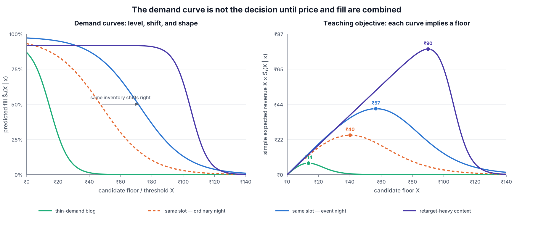
• Level: the thin-demand blog has a low probability of attracting bids even at modest thresholds.
• Shift: the ordinary-night and event-night curves describe the same inventory. Event demand shifts the curve to the right, so the revenue peak moves with it.
• Shape: the retarget-heavy context has a plateau followed by a cliff. That shape is consistent with concentrated high-value demand, but $S_1$ alone cannot prove that one bidder caused it or that no runner-up exists.

If bidder-identity and $B_2$ logs confirm one serious bidder with no meaningful runner-up, a second-price floor just below the cliff can bind and lift payment. Without that additional evidence, the top-bid curve supports only the fill/revenue calculation shown in the right panel. In a first-price auction, even that interpretation requires an estimated bidder response to the floor.

---

7. Production Wrinkles

Six things separate the toy from a production system:

1. Policy-dependent visibility. The SSP observes returned bids, not latent counterfactual bids. Historical floor, routing, eligibility, and timeouts belong in the training audit. Clean floor experiments are the strongest way to learn the response $S_1(X\mid x,\pi_F)$, but a usable design is more than “perturb the floor”: randomize from a pre-approved floor set within inventory strata, log the assignment probability, hold conservative caps and a fallback, and protect latency, fill, user experience, and contractual guarantees. One design caveat matters especially here: naive unit-level A/B is contaminated because bidders adapt and auctions interact - raising one auction’s floor changes the same bidders’ behavior in others - so switchback (time-block) or market-level designs are usually safer than per-request randomization, and both immediate revenue and longer-run participation/shading must be measured before ramping or rolling back.
2. Monotonicity after calibration. Independent per-threshold calibration can reintroduce impossible crossings. Project the calibrated grid onto a decreasing sequence, or use a threshold-conditioned model and a joint monotone calibrator.
3. Class imbalance and probability meaning. High thresholds may have only a few percent positives. Class weighting or oversampling can help optimization but alters the apparent class prior; recalibrate before treating outputs as probabilities.
4. Leakage-safe features and splits. Use only information available before floor selection. Keep every threshold-expanded row for one auction in one fold, use time-based evaluation, and compute target or historical aggregates from past data only.
5. Freshness and uncertainty. There is no universal “days, not months” window. Choose rolling windows or time decay from measured drift and volume, and ship predictions with minimum-support rules or shrinkage toward parent segments.
6. Cold start. A new publisher or slot lacks reliable local history. Fall back hierarchically (category × geo × format, for example) and start with a lower, fill-preserving floor while evidence accumulates.

---

8. The Money and Power Ledgers

As with the rest of the series, the floor decision reads most honestly through two ledgers.

Money ledger. A candidate floor is not chosen on “predicted revenue” as a single number; several distinct quantities sit between the winning bid and the publisher’s bank:

Quantity	Note
Gross winning bid	What the buyer submits
Mechanism payment	Second-price pays $\max(B_2, F)$; first-price pays $B_1$
SSP / exchange / data fees	Deducted before the publisher sees anything
Fallback / passback revenue	$r_0(x)$ recovered on an otherwise-empty auction
Publisher net revenue	The number that actually matters to the seller
Long-run participation effect	A floor that wins today can thin future demand

The last row is the one a short-horizon optimizer forgets: maximizing this week’s net revenue with aggressive floors can teach bidders to shade or leave, lowering the whole curve later.

Data / privacy and power ledger. The good news first: the features that drive these curves are largely contextual - hour, day, geo, device, inventory, lagged partner depth - and demand forecasting rarely needs a persistent per-user identifier. Where audience signals do enter, the questions are the usual ones: are they consented, retained proportionally, and stable enough not to be noise in sparse segments?

The power entry is sharper and specific to floors. A dynamic, individualized floor is, in effect, an estimate of how much a buyer is willing to pay, used to raise the price to them specifically. That can lift short-run publisher revenue, but it also shifts surplus away from buyers in a way that is opaque to them, and it can erode auction transparency and bidder trust - concerns that do not show up anywhere in the revenue formula. The same machinery that makes floors “smart” is the machinery that makes them contestable, and a responsible operator weighs both. (The broader supply-transparency and auction-experimentation questions this raises are threads later articles in the series take up directly.)

9. Recap

The pipeline is:

log context, policy, and returned bid stacks → create nested $B_1$ and $B_2$ threshold labels → split by auction and time → fit and calibrate monotone probability models → score the candidate grid → convert the curve into mechanism-appropriate expected revenue → apply uncertainty and policy guardrails.

The supervision is operationally cheap because labels come from auction outcomes rather than human annotation. But they are not policy-neutral: they describe the demand sources invited and the floors shown when the data was collected.

The object built here, $\Pr(B_1\ge X\mid x)$ as a function of $X$, is the seller-side counterpart of the curve estimated in our bid-landscaping post. The DSP reconstructs a threshold distribution from partial feedback; the SSP reads a much richer returned-bid stack. Same family of curves, different observation regimes, and different reasons to be careful.

References

• IAB Technology Laboratory. OpenRTB 2.x specification (living standard, 2.6 onward).
• Feng, Z., Lahaie, S., Schneider, J. & Ye, J. (2021). Reserve Price Optimization for First Price Auctions in Display Advertising. ICML.
• LightGBM. Parameters: monotone constraints.
• scikit-learn. Probability calibration.