Bid Landscaping: Learning from the Auctions We Lost, with Survival Analysis

Recently, while working for a client in the AdTech domain, I got to understand how Google’s hotel ads mechanism works end to end - how a hotel’s rate surfaces into an auction, how Ad Rank resolves it, and how the advertiser’s bid knob actually connects to the clicks that come out the other side. My task was to design the bid optimization algorithm: given what we know about each auction context, what should we bid?

Digging into that problem, I kept running into the same wall from a different direction each time, and the concept that finally resolved it was bid landscaping. It wasn’t entirely new to me - back at Walmart, while working on improving campaign budget underutilization, I had used bid-landscape win rates as an input to pacing decisions. But that was a consumer’s view of the landscape: a curve someone else had estimated, which I read numbers off. This time I had to build one, and building it forced me to understand where the curve comes from, why the obvious way to estimate it is quietly wrong, and why the correct tool is - of all things - a statistical method from medical survival studies.

This post is that detailed take: what a bid landscape is, why lost auctions are the most misunderstood data we have, and how the Kaplan-Meier estimator turns them into a win curve, worked end to end on a toy dataset.

1. What is a Bid Landscape?

A bid landscape (also called a win curve) is a function:

\[W(b) = P(\text{we win the auction} \mid \text{we bid } b)\]

Before going further, two prices need to be pinned down, because confusing them derails everything downstream:

• $b$ - our bid. The amount we submit to the auction; the lever we control. In the landscape $W(b)$ it is the x-axis: “if we were to bid $b$…”.
• $P$ - the winning threshold. The minimum effective bid we would have needed to win that auction. It is not our bid; it is a property of the auction, set by everything we don’t control - competitors’ bids, their quality scores, reserve prices - and different every time.

We win an auction iff $b \ge P$. In a textbook second-price auction, $P$ is simply the highest competing bid (the clearing price), and it is also what we pay on a win. Real platforms are messier: Ad Rank folds in quality, reserves set floors, and much of RTB now runs first-price. To isolate the statistical problem, this article assumes the clean second-price case - winning reveals $P$ exactly (we paid it), losing reveals only that $P > b$. Everything that follows depends only on that observation structure, so it survives the platform messiness; only the “what we pay” bookkeeping changes with the mechanism.

The win curve is monotonically increasing - bid more, win more - and it is the missing half of the bidding problem. Most bid optimization pipelines model the value side well: pCTR, pCVR, expected revenue per click. The bid landscape is the cost side: what does it take to actually win, and what will winning cost?

\[\text{profit}(x, b) = \underbrace{\text{value}(x)}_{\text{from won clicks}} - \underbrace{\text{cost}(x, b)}_{\text{from the landscape}}\]

Here $x$ is the auction context - the bundle of features describing the particular auction we are bidding into: query, device, geography, time of day, placement, and so on. The value of winning depends on the context alone; the cost of winning depends on the context and on how much we bid. Everything in this article - the win curve, the toy example, the pacing math - is implicitly per-context: one landscape for each segment of comparable auctions, a point section 8 returns to.

A bidder that models only value is competition-blind. It knows what an impression is worth but has no idea what the market charges for it.

2. The Problem: We Only Observe Half the Story

Here is what a typical auction log gives us:

Auction outcome	What we observe about the clearing price
Won	The exact price $P$ (we paid it)
Lost	Only that $P > \text{our bid}$

The tempting shortcut is to estimate the price distribution from won auctions only - after all, those are the only rows with an actual price in them. This is exactly the wrong move, and the reason is selection bias: we only ever observe prices below our historical bids. The entire upper region of the distribution - the prices that beat us - is systematically missing from our sample.

This is the classic WWII bomber problem. The military examined returning planes, mapped where the bullet holes were, and proposed armoring those spots - until Abraham Wald pointed out that they were only studying the planes that came back. The holes they could see were, by definition, the survivable ones. Estimating competing prices from won auctions is studying the planes that returned.

An even cruder shortcut is:

\[\hat{W} = \frac{\text{auctions won}}{\text{total auctions}}\]

which produces a single flat number - “we win 50% of the time” - with no dependence on the bid at all. It punishes our win-rate estimate at \$5 with auctions we lost at \$3, even though those losses say nothing about our ability to win at \$5. We will see this fail concretely on the toy dataset below.

So the situation is: lost auctions clearly carry information (“the price was higher than \$X” is a real fact about the competition), but we can’t use them naively, and we can’t drop them without bias. We need machinery built for partial observations.

That machinery exists. It just lives in a different field.

3. A Detour Through the Hospital: Survival Analysis

Picture a waiting room full of patients, each having entered at a different time. Periodically a name is called - the event happens (in the medical original, something like death or relapse). But some patients leave before their name is called, and for them we know something real but incomplete: they waited at least this long, but we don’t know how long they would have waited.

Every subject in a survival study is therefore one of two types:

Subject	What happens	Statistical term
Name is called	The event occurs, at an observed time	Event
Leaves early	Observation stops before the event	Censored (right-censored)

The defining challenge of survival analysis is what to do with the censored subjects, and the key insight is that we cannot do either of the two obvious things:

• We can’t drop them. The patients who leave uncalled tend to be the ones who lasted longest. Discarding them biases survival estimates downward.
• We can’t count them as events. Their event never happened while observed. Pretending it did biases the estimate even more.

The Kaplan-Meier estimator is the tool that uses these incomplete records correctly - keeping each subject in the “still at risk” pool for exactly as long as it was observed, then quietly removing it, never inventing an event that wasn’t seen.

If the phrase “we know it was more than X, but not how much more” is ringing a bell, it should.

4. An Auction Is a Survival Problem

Map the waiting room onto the auction log. The quantity that plays the role of survival “time” is the clearing price $P$ - the competition’s price, not our bid:

Survival analysis	Our auction problem
Subject (a patient)	One auction
“Time” $T$	Clearing price $P$
Event observed at $T$	We win → we pay $P$ → we observe $P$ exactly
Right-censored at $c$	We lose → we only know $P > \text{our bid}$ → censored at our bid
Survival function $S(t) = P(T > t)$	$S(b) = P(P > b)$ = probability we lose at bid $b$

Two things to lock in:

• A win is a fully-observed data point. We paid the clearing price, so we know $P$ exactly.
• A loss is a censored data point. We only learn $P > b$. We never see the lost price - and we don’t need to. The bid alone is the censoring point. The lost price being invisible is the expected state of the data, not a blocker.

And the curve we want falls straight out:

\[W(b) = P(\text{win at bid } b) = P(P \le b) = 1 - S(b)\]

If Kaplan-Meier gives us $S$ (the loss curve), the win curve is just $1 - S$.

5. The Kaplan-Meier Estimator, Piece by Piece

To compute KM we sweep a candidate bid $b$ upward from zero and, at each price where we observed a win, step the curve down a little. Four quantities drive it:

• Event price $t_i$ - a price at which we observed a win (a fully-observed clearing price). These are the only prices where the curve moves.
• Number of events $d_i$ - how many auctions cleared at exactly $t_i$ (how many wins landed at that price).
• Risk set $n_i$ - how many auctions are still unresolved just before price $t_i$: the ones we can still vouch for having a threshold $\ge t_i$. An auction is in the risk set at $t_i$ if its recorded value (its win-price if won, its bid if lost) is $\ge t_i$. There are two ways to have left the pool before $t_i$:
  • A win at a price below $t_i$ is resolved - its threshold is known exactly, and it is lower. It has nothing left to say about $t_i$.
  • A loss at a bid below $t_i$ leaves for a subtler reason. All we know about it is “threshold > its bid” - whether its threshold reaches $t_i$ or stopped somewhere in between is unknowable, because our information about it ran out at its bid. Keeping it in the pool at $t_i$ would amount to claiming its threshold is $\ge t_i$, which we cannot vouch for. So it exits at the last price where we can vouch for it: its own bid.
• Censored count $c_i$ - losses recorded at that value. These do not move the curve, but they shrink the risk set for all higher prices - we stop tracking that auction past its bid.

The intuition before the formula

Let’s freeze at a single event price $t_i$ and look only at the risk set: $n_i$ auctions whose thresholds are all known to be at least $t_i$. Of those, $d_i$ just resolved - their threshold turned out to be exactly $t_i$. So the ratio

\[\frac{d_i}{n_i} = \hat{P}\big(\text{threshold} = t_i \;\big|\; \text{threshold} \ge t_i\big)\]

is the estimated chance that an auction’s threshold resolves at this price rung, given that it climbed this far. (Survival analysis calls this the hazard at $t_i$.) Its complement,

\[1 - \frac{d_i}{n_i} = \hat{P}\big(\text{threshold} > t_i \;\big|\; \text{threshold} \ge t_i\big)\]

is the chance of getting past the rung. Picture the sweep upward as a climb: each event price asks the auctions still climbing one question - “did your threshold resolve here?” - and $1 - d_i/n_i$ is the fraction that answered no and kept climbing.

The estimator simply chains these rung-survival probabilities together:

\[\hat{S}(b) = \prod_{t_i \le b} \left(1 - \frac{d_i}{n_i}\right)\]

Why a product?

Read $S(b)$ as “the threshold survives past $b$” - i.e., “we would still lose at bid $b$.” To survive past $b$, the threshold must get past every event price along the way, so the chain rule of probability multiplies the conditional pieces:

\[S(b) = P(\text{survive past } t_1) \cdot P(\text{survive past } t_2 \mid \text{survived } t_1) \cdots\]

and each conditional factor is exactly the rung-survival probability $1 - d_i/n_i$ we just built.

Censored losses never contribute a factor - they aren’t events. They only lower $n_i$ for later prices, which is exactly how a “we know it’s bigger than X” observation should count. That one sentence is the whole reason KM is the right tool: a lost auction with no known price still pulls its weight, through the risk set, without us ever inventing its price.

The data KM fits on

Concretely, every auction $i$ contributes one row with two fields (plus the context columns that define the segment):

\[Y_i = \begin{cases} P_i & \text{if won (the price we paid)} \\ B_i & \text{if lost (our bid)} \end{cases} \qquad \delta_i = \begin{cases} 1 & \text{if won} \\ 0 & \text{if lost} \end{cases}\]

KM is fitted on $(Y_i, \delta_i)$ - a duration-like value and an event flag, the exact shape every survival library expects. No lost price appears anywhere in the schema.

6. Worked Example: Eight Auctions

One context - say, a single ad-group on mobile. For each auction we logged our bid and the outcome. On wins we also see the price we paid (the clearing price, since this is second-price); on losses we see nothing but our own bid.

Auction	Our bid	Outcome	Clearing price seen	KM “value”	KM type
1	\$5	win	\$2	2	event
5	\$4	win	\$3	3	event
3	\$3	lose	- (only know > \$3)	3	censored
8	\$4	lose	- (only know > \$4)	4	censored
4	\$6	win	\$5	5	event
7	\$6	win	\$5	5	event
2	\$5	lose	- (only know > \$5)	5	censored
6	\$7	lose	- (only know > \$7)	7	censored

$n = 8$ auctions: 4 wins (events) and 4 losses (censored). Note that we win at or below our bid (we pay the second price) and we lose above our bid.

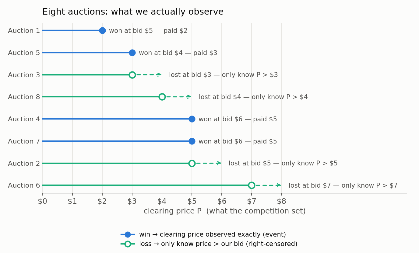
Tie convention: when an event and a censored observation share the same value (here, value 5 has 2 wins and 1 loss), the censored one is treated as occurring just after the events - so it is still counted in the risk set at that event price, then removed afterward.

The computation, step by step

Sort everything by value and walk upward. The risk set $n$ at each price is the number of auctions whose recorded value is $\ge$ that price.

Price 2 - 1 win, 0 losses. Risk set = all 8 (every value $\ge 2$).

\[S(2) = 1 - \tfrac{1}{8} = 0.875\]

Price 3 - 1 win (auction 5) + 1 loss (auction 3). Risk set = 7 (everyone except auction 1, whose price of 2 is already resolved).

\[S(3) = 0.875 \times \left(1 - \tfrac{1}{7}\right) = 0.875 \times \tfrac{6}{7} = 0.750\]

After this price, auction 5 (event) and auction 3 (censored) leave the pool.

Price 4 - 0 wins, 1 loss (auction 8). Risk set = 5. No event ⇒ the curve does not step. The loss just removes auction 8 going forward.

\[S(4) = 0.750 \quad (\text{unchanged})\]

Price 5 - 2 wins (auctions 4, 7) + 1 loss (auction 2). Risk set = 4 (auctions 2, 4, 6, 7 remain).

\[S(5) = 0.750 \times \left(1 - \tfrac{2}{4}\right) = 0.750 \times 0.5 = 0.375\]

After this, auctions 4 and 7 (events) and auction 2 (censored) leave. Only auction 6 remains.

Price 7 - 0 wins, 1 loss (auction 6). Risk set = 1. No event ⇒ no step.

\[S(7) = 0.375 \quad (\text{unchanged})\]

The full table

Price $t$	Risk set $n$	Wins $d$	Losses $c$	Step $1 - d/n$	$S(t)$ = lose prob	$W(t) = 1 - S(t)$ = win prob
2	8	1	0	7/8	0.875	0.125
3	7	1	1	6/7	0.750	0.250
4	5	0	1	-	0.750	0.250
5	4	2	1	2/4	0.375	0.625
7	1	0	1	-	0.375	0.625

The bid landscape we just built

Reading off the win curve $W(b)$ (a right-continuous step function):

\[W(b) = \begin{cases} 0.000 & b < 2 \\ 0.125 & 2 \le b < 3 \\ 0.250 & 3 \le b < 5 \\ 0.625 & b \ge 5 \ \ (\text{known only up to } \$7) \end{cases}\]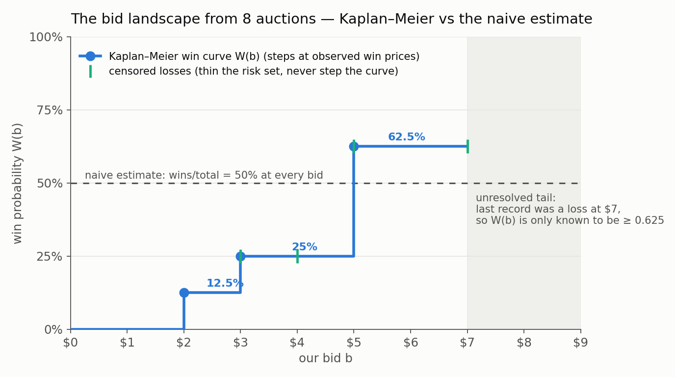

How to use it:

• Bid $\rightarrow$ win rate: bid \$5 $\Rightarrow$ ~62.5% win probability; bid \$3 $\Rightarrow$ ~25%.
• Target win rate $\rightarrow$ bid: want ~25% coverage? Bid ~\$3. Want ~62%? Bid ~\$5.
• Spend curve: under second-price, when we win at bid $b$ we pay the clearing price ($\le b$). The expected cost per win comes from the KM curve itself - worked out next, because there is a trap in it.

From KM jumps to expected cost

The steps of $\hat{F}(b) = 1 - \hat{S}(b)$ are not just a picture - each jump is a probability mass sitting at an observed win price:

\[\hat{p}_i = \hat{F}(t_i) - \hat{F}(t_i^-)\]

From our table: mass $0.125$ at \$2, $0.125$ at \$3, $0.375$ at \$5. The expected cost per win at bid $b$ weights the event prices by these masses:

\[\mathbb{E}[P \mid P \le b] = \frac{\sum_{t_i \le b} t_i \, \hat{p}_i}{\hat{F}(b)}\]

At $b = 5$:

\[\mathbb{E}[P \mid P \le 5] = \frac{2(0.125) + 3(0.125) + 5(0.375)}{0.625} = \frac{2.5}{0.625} = \$4.00\]

The trap: averaging the observed win prices directly - $\{2, 3, 5, 5\}$, giving \$3.75 - is wrong for the same reason the naive win rate was wrong. It weights by the won sample, in which the \$5 wins are underrepresented (the losses at \$3 and \$4 thinned the pool exactly there). The KM masses undo that distortion, and the corrected cost is higher. Combine win-rate × cost-per-win × volume and we have $\text{spend}(b)$, which is what a budget-pacing loop needs.

Why this beats the naive estimate

The naive “wins/total = 4/8 = 50% at any bid” answer is visibly wrong in the figure: it understates the win rate at \$5 and overstates it at \$3. KM fixes this precisely through the risk set. The loss at bid \$3 (auction 3) and the loss at bid \$4 (auction 8) leave the pool below \$5, so they never drag down $S(5)$. Each point on the curve uses only the auctions that are genuinely informative at that bid - which is why KM gives a clean 62.5% at \$5 rather than a muddied 50%.

One honesty note before moving on: 62.5% from eight auctions is mechanics, not measurement. KM comes with standard uncertainty estimates (Greenwood’s formula), and at $n = 8$ the confidence band would be embarrassingly wide. The toy exists to show the machinery. In production, landscape numbers should ship with intervals, minimum-volume thresholds, or shrinkage toward a broader parent segment before anyone bids real money on them.

The same computation in code

The entire worked example is a few lines with any survival library (lifelines here). The only modeling decision is the encoding from the schema above: duration = price if won, bid if lost; the event flag = won.

import numpy as np
import pandas as pd
from lifelines import KaplanMeierFitter

# The eight auctions from the worked example
auctions = pd.DataFrame({
    "bid":   [5, 4, 3, 4, 6, 6, 5, 7],
    "won":   [True, True, False, False, True, True, False, False],
    "price": [2, 3, np.nan, np.nan, 5, 5, np.nan, np.nan],  # seen only on wins
})

duration = np.where(auctions["won"], auctions["price"], auctions["bid"])
event = auctions["won"].astype(int)          # 1 = event (win), 0 = censored

kmf = KaplanMeierFitter()
kmf.fit(duration, event_observed=event)

win_curve = 1 - kmf.survival_function_["KM_estimate"]    # W(b) = 1 - S(b)

# CDF jumps are probability masses -> expected cost per win at bid b
masses = win_curve.diff().fillna(win_curve)
def expected_cost_per_win(b):
    m = masses[masses.index <= b]
    return (m.index * m).sum() / win_curve[win_curve.index <= b].max()

Running it reproduces the table exactly: $W(5) = 0.625$ and expected cost per win at \$5 = \$4.00. In production the same ten lines run per segment (stratified by the context columns), not once globally - for reasons the caveats below make concrete.

7. From Win Curve to Budget-Aware Bidding and Pacing

Here is where the landscape earns its keep in a bid optimizer - though not where it is usually assumed to. A profit-maximizing bidder wants, for each auction context $x$ with estimated value $v(x)$:

\[\Pi(\theta) = \sum_x N(x) \cdot \mathbb{E}_{P}\Big[ \big(v(x) - P\big) \cdot \mathbb{1}\{\text{Bid}(x;\theta) \ge P\} \Big]\]

The expectation is over the distribution of winning thresholds - and that distribution, $F(p) = W(p)$, is exactly what the landscape estimates. With it, the objective becomes computable for any candidate bid, not just the ones we historically placed:

\[\Pi(\theta) = \sum_x N(x) \int_0^{\text{Bid}(x;\theta)} \big(v(x) - p\big) \, f(p) \, dp\]

where $f(p)$ is the density implied by the KM curve.

First, an honest disclaimer: where the landscape changes nothing

In an idealized second-price auction with no constraints, the landscape does not change the per-auction bid. Differentiate the per-auction objective:

\[\frac{d\Pi(b)}{db} = \big(v - b\big) \, f(b)\]

This is positive for $b < v$ and negative for $b > v$ wherever $f(b) > 0$, so $b^* = v$: bid the value, whatever the competition looks like. That is the classic truthful-bidding result. The landscape moves the expected profit and volume at that bid - it does not move the bid.

So why estimate it at all? Because no production system lives in that idealized world. The landscape starts driving decisions the moment any of the following enters - and at least one always does.

1. Budgets and pacing. With a budget, we can no longer afford to win everything worth winning; spend needs a price. Put a Lagrange multiplier $\lambda$ on spend and the per-auction problem becomes

\[\max_b \int_0^b \big(v - (1 + \lambda)\, p\big) \, f(p) \, dp \quad \Rightarrow \quad b^* = \frac{v}{1 + \lambda}\]

The form of the answer is still “bid a scaled value” - but choosing $\lambda$ requires exactly what the landscape provides: $\text{spend}(\lambda)$ curves per segment, so the budget lands where the market is cheapest per unit of value. This is the use I first met at Walmart, working on campaign budget underutilization: “how much more volume does a 10% bid increase buy?” is a question about the slope of the win curve, and pacing tolerates a coarse landscape, which makes it the ideal first consumer of one.

2. Counterfactual / off-policy evaluation. Before deploying a new bidding policy, the landscape predicts its win rate, spend, and profit offline. One discipline applies: this works for bids inside the support of our data. Asking $W($4.50)$ when our observations span \$2-\$7 is interpolation; asking what happens at \$55 when our bids never exceeded \$50 is tail extrapolation, and non-parametric KM is flat and silent past its last observation (caveat 1 below). The landscape evaluates counterfactuals we have evidence about, not arbitrary ones.

3. First-price auctions and bid shading. Where we pay our own bid, truthful bidding is no longer optimal: the shading trade-off $\max_b F(b)\,(v - b)$ depends directly on the shape of $F$. Every shading decision is a landscape read. The same goes for ROI and CPA constraints, bid floors and caps, and knowing when to sit out because expected cost exceeds value.

And the point worth stating precisely: the $F(p)$ inside all of these is censoring-aware - lost auctions participate as censored observations shrinking the risk set, which removes the specific survivorship bias of discarding losses. That is not the same as unbiased: censoring-awareness alone does not cure confounded bids, policy drift, or context mixing; those need the assumptions in the next section. (This censoring-aware view of bid landscapes is well established in the RTB literature - it underpins bid-aware gradient descent from KDD 2016 and the Deep Landscape Forecasting model from KDD 2019, which wires KM-style survival reasoning into an RNN.)

8. Reading the Curve Honestly: Caveats

A KM bid landscape is only as trustworthy as the data feeding it. Five things to respect:

1. The tail is unresolved. Our highest record (auction 6 at \$7) was a loss - censored. The curve never reaches 1.0 and we have literally no evidence about prices above \$7; the win curve is only known to be ≥ 0.625 there. To learn the top of the curve, we must occasionally bid higher.

2. We need bid spread to trace the curve. If every auction had been bid at exactly \$5, we’d know $W($5)$ - one point, not a curve. Variation in bids (across time, across contexts, or via deliberate exploration) is what fills the landscape in.

3. Endogeneity is the make-or-break. KM assumes the censoring point (our bid) is independent of the clearing price - non-informative censoring. In reality we bid high exactly where and when we judge value high, which often correlates with stiffer competition. Fit naively on such observational data and we get a biased, too-flat curve (“bid more, didn’t win proportionally more” - because competition was also higher then). The highest-leverage mitigation is a small exploration budget: randomly perturb the deployed bid by ±ε on a slice of traffic. That gives clean, unconfounded variation and turns the landscape from suggestive into trustworthy. If we do one thing, do this. One refinement for production: the assumption we actually need is not unconditional independence ($P \perp B$) but conditional independence ($P \perp B \mid X$) - after conditioning on the auction context $X$ (device, geography, property, time of day), our bid should carry no additional information about the threshold. That is the real argument for estimating landscapes per segment, and it trades directly against caveat 5: condition on too much context and every segment becomes too sparse to estimate.

4. Match the estimator to what we actually log. The worked example assumed we observe the price paid on wins - textbook right-censored KM. If we only have a win/loss flag per auction (no prices), the data is “current-status” and the correct tool is isotonic regression / NPMLE (pool-adjacent-violators on the win indicator vs bid) - same spirit, a monotone win curve, but different machinery that leans much harder on bid spread. If we log CPC paid on wins, upgrade to proper KM; it is strictly better.

5. Sparsity and non-stationarity. Estimate at a coarse enough grain to have volume (ad-group, or property × device - not the full joint context), over a window short enough that competition hasn’t shifted, and re-estimate on a slow loop. Competitors adapt; a landscape is a perishable artifact, never a frozen one.

One more practical note from the hotel-ads world: some platforms won’t give us auction-level win/loss logs at all, but expose a bid simulator instead - a per-criterion curve of estimated clicks, cost, and impressions at alternative bids. In our language, that is an operational analogue of the landscape, pre-built by the platform from the full auction data we never see - including the lost auctions and the competitors’ bids. One caution on reading it: $\text{clicks}(b)$ is not literally the win curve. Clicks fold together eligibility, auction wins, position effects, and click-through - roughly $N \cdot P(\text{win} \mid b) \cdot \mathbb{E}[\text{CTR} \mid \text{won}, b]$ - so simulator curves are downstream response curves, one step removed from the pure auction-level $W(b)$. They still serve the pacing and counterfactual jobs well. Using them largely sidesteps the endogeneity problem in caveat 3, at the price of inheriting a model we cannot audit - so backtest the simulator’s predicted point against our realized clicks and cost before trusting it for budget decisions.

Choosing the estimator by what we log

The right tool follows mechanically from the feedback the platform gives us:

Logged feedback	Right tool
Price paid on wins + our bid on losses	Kaplan-Meier (this article)
Only a win/loss flag at our bid	Current-status NPMLE / isotonic regression
Exact market price for every auction	Plain empirical CDF - no censoring machinery needed
High volume + rich context	Conditional survival models (below)
Strong temporal drift	Rolling / time-weighted re-estimation

And when a single per-segment curve stops being enough, there is a natural ladder to climb, each rung buying more context-sensitivity at the price of more data and more assumptions: global KM, then stratified KM (one curve per segment), then semi-parametric conditional models (Cox, accelerated failure time), then tree ensembles (random survival forests, gradient-boosted survival), and finally neural conditional models like Deep Landscape Forecasting. Climb only as far as volume supports. The toy in this article is rung one - and rung one estimated correctly beats rung five fed with wishful data.

9. Recap

Treat each auction as a survival “subject” whose event is the clearing price. A win reveals that price exactly (an event); a loss reveals only that the price exceeded our bid (right-censored at the bid - no lost price needed). Kaplan-Meier multiplies, at each observed win-price, the conditional chance of “not yet winning” - $(n_i - d_i)/n_i$ - using a risk set that censored losses quietly shrink. The result is $S(b)$, and $W(b) = 1 - S(b)$ is the bid landscape: the win probability at any bid, learned from every auction, won or lost.

The medical statisticians who built this machinery in 1958 were trying not to lie about patients who left the study early. It turns out the same discipline - refusing to invent data we didn’t observe, while refusing to throw away the partial information we did - is exactly what separates a bid optimizer that learns from the full market from one that studies only the planes that came back.

References

• Kaplan, E. L. & Meier, P. (1958). Nonparametric Estimation from Incomplete Observations. JASA.
• Zhang, W. et al. (2016). Bid-aware Gradient Descent for Unbiased Learning with Censored Data in Display Advertising. KDD 2016.
• Ren, K. et al. (2019). Deep Landscape Forecasting for Real-time Bidding Advertising. KDD 2019. (arXiv:1905.03028)
• Ghosh, A. et al. (2019). Scalable Bid Landscape Forecasting in Real-time Bidding. ECML-PKDD 2019. (arXiv:2001.06587)