The Wisdom of Trees: From Single Decisions to Ensemble Intelligence

The Ultimate Guide to Decision Trees: From Movie Night Dilemmas to Mathematical Rigor

Imagine playing a game of “20 Questions.” You are trying to guess an object, and you can only ask yes/no questions. To win quickly, you wouldn’t ask, “Is it a 1994 Ford Taurus?” right away. You’d ask broad questions to narrow down the possibilities efficiently: “Is it alive?”, “Is it bigger than a breadbox?”

A Decision Tree is essentially a machine learning algorithm playing an optimized version of “20 Questions” with your data.

1. High-Level Definition and CART

At a high level, a decision tree is a supervised learning algorithm used for both classification (predicting a category, like “Watch” or “Skip”) and regression (predicting a number, like a movie rating).

It works by breaking down a dataset into smaller and smaller subsets while at the same time an associated decision tree is incrementally developed. The final result is a tree with decision nodes and leaf nodes. A decision node (e.g., “Is the lead actor Ryan Reynolds?”) has two or more branches, representing values for the attribute tested. Leaf node (e.g., “Watch”) represents a final decision or prediction.

The Standard: CART (Classification and Regression Trees)

While there are several types of decision trees (like ID3 or C4.5), the modern standard implemented in most libraries (like Python’s scikit-learn) is the CART algorithm.

Crucially, CART trees create binary splits. This means every question must have exactly two answers (Yes/No, True/False, or Less than/Greater than). Even if a category has three options (e.g., Action, Comedy, Drama), CART won’t split it three ways at once. It will ask something like: “Is it Action vs. NOT Action (Comedy/Drama)?”

2. The Dataset: The Movie Night Dilemma

To understand the math, we need data. Let’s try to predict two things: whether we will Watch a movie (Classification) and what Rating (out of 10) we might give it (Regression).

Here is our dataset of 15 movies:

Movie ID	Lead Actor	Genre	Duration (mins)	Target 1: Watched? (Class)	Target 2: Rating (Reg)
1	Ryan Reynolds	Comedy	95	Yes	8.5
2	Ryan Reynolds	Action	110	Yes	8.0
3	Ryan Reynolds	Comedy	105	Yes	9.0
4	Ryan Reynolds	Drama	130	No	6.5
5	Ryan Reynolds	Action	125	Yes	7.5
6	Meryl Streep	Drama	140	Yes	9.5
7	Meryl Streep	Drama	160	Yes	9.0
8	Meryl Streep	Comedy	110	No	7.0
9	Meryl Streep	Drama	135	Yes	8.5
10	Meryl Streep	Action	120	No	6.0
11	Keanu Reeves	Action	115	Yes	8.5
12	Keanu Reeves	Sci-Fi	150	Yes	9.0
13	Keanu Reeves	Sci-Fi	100	Yes	8.0
14	Keanu Reeves	Drama	145	No	5.5
15	Keanu Reeves	Action	135	No	7.0

Summary Stats:

• Total Samples ($N$): 15
• Watched = Yes: 9 ($p_{yes} = 9/15 = 0.6$)
• Watched = No: 6 ($p_{no} = 6/15 = 0.4$)

3. The Algorithm Step-by-Step (Defining the Math)

The core idea of decision tree building is greedy recursive partitioning.

• Greedy: At each step, pick the single best split right now, without worrying about future steps.
• Recursive Partitioning: Take a dataset, split it into two based on a rule, then repeat the process on the two resulting smaller datasets.

The goal is to create “pure” leaf nodes. For classification, a pure node contains only one class (e.g., 100% “Yes”). For regression, a pure node contains values that are all very close to each other (low variance).

How do we measure “purity”? We measure the opposite: Impurity.

Classification Metrics: Entropy and Gini

For a node $S$ with classes $i=1$ to $C$, where $p_i$ is the proportion of items belonging to class $i$:

1. Entropy (A measure of disorder/uncertainty) A classic concept from information theory. It ranges from 0 (perfectly pure) to $\log_2(C)$ (maximum disorder). For a binary classification (Yes/No), max entropy is 1 (a 50/50 split).

\[Entropy(S) = - \sum_{i=1}^{C} p_i \log_2(p_i)\]

Note: By convention, $0 \log_2(0) = 0$.

2. Gini Impurity (Probability of misclassification) A measure of how often a randomly chosen element from the set would be incorrectly labeled if it were randomly labeled according to the distribution of labels in the subset. It ranges from 0 (perfectly pure) to 0.5 (maximum impurity for binary classification). It’s generally faster to compute than log-based entropy.

\[Gini(S) = 1 - \sum_{i=1}^{C} (p_i)^2\]

3. Information Gain (The Deciding Factor) To decide which feature to split on, we calculate the potential Information Gain (IG). IG is simply the impurity of the parent node minus the weighted average impurity of the child nodes created by the split. We want the split that maximizes IG.

\[IG(Split) = Impurity(Parent) - \left[ \frac{N_{Left}}{N_{Parent}} \times Impurity(Left) + \frac{N_{Right}}{N_{Parent}} \times Impurity(Right) \right]\]

Regression Metric: Variance Reduction

For regression, we can’t use classes. Instead, we want the numerical values in a node to be clustered tightly around the average. We use Variance (or Mean Squared Error - MSE) as our measure of impurity.

\[Variance(S) = \frac{1}{N} \sum_{j=1}^{N} (y_j - \bar{y})^2\]

Where $y_j$ is an individual target value and $\bar{y}$ is the mean of values in that node.

The goal in regression is to maximize Variance Reduction, calculated exactly the same way as Information Gain above, just replacing entropy/gini with variance.

4. Running the Algorithm (Exact Calculations)

Let’s build the first node of our classification tree (Target: “Watched?”). We need to find the best split among Actor, Genre, and Duration.

Step 0: Calculate Baseline Impurity of the Whole Dataset (Parent Node)

• 9 Yes, 6 No ($p_{yes}=0.6, p_{no}=0.4$)
• Base Entropy: $- (0.6 \log_2 0.6 + 0.4 \log_2 0.4) \approx - (-0.442 - 0.529) = \textbf{0.971}$
• Base Gini: $1 - (0.6^2 + 0.4^2) = 1 - (0.36 + 0.16) = 1 - 0.52 = \textbf{0.48}$

Candidate Split 1: Categorical Feature (Lead Actor)

CART needs a binary split. Let’s test: “Is Lead Actor == Ryan Reynolds?”

• Left Child (True - Reynolds): Total 5 movies.
  • Watched: 4 Yes, 1 No ($p_{yes}=0.8, p_{no}=0.2$)
• Right Child (False - Not Reynolds): Total 10 movies (Streep + Reeves).
  • Watched: 5 Yes, 5 No ($p_{yes}=0.5, p_{no}=0.5$)

Calculation using Entropy:

1. Entropy(Left): $- (0.8 \log_2 0.8 + 0.2 \log_2 0.2) \approx \textbf{0.722}$
2. Entropy(Right): $- (0.5 \log_2 0.5 + 0.5 \log_2 0.5) = \textbf{1.0}$ (Maximum disorder!)
3. Weighted Impurity of Children: $(\frac{5}{15} \times 0.722) + (\frac{10}{15} \times 1.0) = 0.241 + 0.667 = \textbf{0.908}$
4. Information Gain (Entropy): $0.971 (\text{Base}) - 0.908 (\text{Children}) = \textbf{0.063}$

Calculation using Gini Impurity:

1. Gini(Left): $1 - (0.8^2 + 0.2^2) = 1 - (0.64 + 0.04) = \textbf{0.32}$
2. Gini(Right): $1 - (0.5^2 + 0.5^2) = 1 - (0.25 + 0.25) = \textbf{0.50}$
3. Weighted Impurity of Children: $(\frac{5}{15} \times 0.32) + (\frac{10}{15} \times 0.50) = 0.107 + 0.333 = \textbf{0.44}$
4. Information Gain (Gini): $0.48 (\text{Base}) - 0.44 (\text{Children}) = \textbf{0.04}$

We would repeat this for “Actor == Streep” and “Actor == Reeves” to find the best Actor split.

Candidate Split 2: Numerical Feature (Duration)

How does a tree split continuous numbers like duration? It tests “thresholds.”

1. Sort the unique durations: 95, 100, 105, 110, 115, 120, 125, 130, 135, 140, 145, 150, 160.
2. Use the midpoints between values as candidate splits: 97.5, 102.5, 107.5, etc.

Let’s test the split: “Duration < 117.5?” (Midpoint between 115 and 120).

• Left Child (Duration < 117.5): Movies 1, 2, 3, 8, 11, 13. Total 6 movies.
  • Watched: 5 Yes, 1 No ($p_{yes} \approx 0.83, p_{no} \approx 0.17$)
• Right Child (Duration >= 117.5): The remaining 9 movies.
  • Watched: 4 Yes, 5 No ($p_{yes} \approx 0.44, p_{no} \approx 0.56$)

Let’s calculate IG using Gini for this split:

1. Gini(Left): $1 - ((5/6)^2 + (1/6)^2) = 1 - (0.694 + 0.028) = \textbf{0.278}$
2. Gini(Right): $1 - ((4/9)^2 + (5/9)^2) = 1 - (0.198 + 0.309) = \textbf{0.493}$
3. Weighted Impurity: $(\frac{6}{15} \times 0.278) + (\frac{9}{15} \times 0.493) = 0.111 + 0.296 = \textbf{0.407}$
4. Information Gain (Gini): $0.48 (\text{Base}) - 0.407 (\text{Children}) = \textbf{0.073}$

The Winner and Full Tree Construction

Comparing the Gini IG of the actor split (0.04) vs. the duration split (0.073), the duration split is currently winning.

The algorithm calculates the IG for every possible binary actor split, genre split, and duration threshold split.

Let’s assume after checking everything, the best first split is Duration < 117.5.

• Node 1 (Root): Duration < 117.5?
  • True Branch (Left): Contains 6 movies (mostly watched). The algorithm repeats the process on this subset. Perhaps it splits next on “Genre == Comedy”.
  • False Branch (Right): Contains 9 movies (mixed). The algorithm repeats the process here. Perhaps it splits on “Actor == Meryl Streep”.

The process stops when a node is 100% pure, or we hit a predefined limit (like maximum depth).

5. Inference: Making Predictions

We have a trained tree. A new movie comes along: Lead Actor: Keanu Reeves, Genre: Sci-Fi, Duration: 110.

Classification Inference (“Watched?”) We drop the data point down the tree. It passes through decision nodes based on its features.

1. Is Duration < 117.5? Yes (110 < 117.5). Go Left.
2. Next question… (e.g., Is Genre == Comedy? No. Go Right).
3. Arrival at Leaf Node.

• Pure Leaf: If the leaf node contains [5 Yes, 0 No] training examples, the prediction is “Yes”.
• Impure Leaf: If the leaf contains [4 Yes, 1 No], the prediction is the majority class: “Yes”. Usually, models also output the probability: $P(Yes) = 4/5 = 80\%$.

Regression Inference (“Rating”) The process is identical, but the final prediction is different. If the new movie lands in a leaf node that contains training movies with ratings of [8.5, 9.0, 8.0], the prediction is the average: $(8.5+9.0+8.0)/3 = \textbf{8.5}$.

6. Overfitting: The Curse of the Decision Tree

Decision trees are notorious for overfitting. Why? Because they are “non-parametric” and can grow indefinitely complex. If allowed, a tree could keep splitting until every single training example has its own leaf node.

A fully grown tree has memorized the training data perfectly (0% training error) but has learned the noise in the data rather than the signal. It will perform terribly on new movies.

How to Prevent Overfitting

We prevent this using Regularization (constraints) or Pruning.

1. Pre-Pruning (Constraints during build time):

• Max Depth: Stop the tree from growing deeper than, say, 3 levels.
• Min Samples Split: Only allowed to split a node if it has at least, say, 5 samples.
• Min Samples Leaf: A split is only valid if the resulting left and right children both have at least, say, 3 samples.
• Max Leaf Nodes: Cap the total number of terminal nodes.

2. Post-Pruning (Cleaning up afterward): Grow the tree to its maximum extent, then start from the bottom and cut off (prune) branches that don’t provide significant predictive power on a validation set (Cost-Complexity Pruning).

7. Decision Boundaries

How does a decision tree view the world?

Because every split is a hard binary threshold on a single feature (e.g., Duration < 117.5), decision trees create orthogonal, axis-parallel decision boundaries.

If you plotted “Duration” vs. another numerical feature, the decision boundary wouldn’t be a smooth curve or a diagonal line. It would look like a series of stairs or rectangular boxes.

While individual boundaries are linear (straight lines), the combination of many such splits allows the tree to approximate highly non-linear relationships.

8. Determining Variable Importance

One of the best features of decision trees is interpretability. We can measure how important each feature was.

Variable importance is calculated by summing up the Information Gain (or Variance Reduction) brought by a specific feature across all nodes where it was used to split.

If “Duration” was used three times in the tree, and those splits cleaned up the data significantly (high IG weighted by the number of samples involved), it will have high importance. These scores are usually normalized so they sum to 1 (or 100%).

In our movie example, if Duration splits consistently separated “Yes” from “No” better than Actor, Duration would have a higher variable importance score.

9. Handling Missing Data

What if we don’t know the duration of a movie?

The Scikit-Learn Reality: The standard CART implementation in scikit-learn does not handle missing values natively. You must handle them before training (e.g., imputing with the mean duration or a placeholder value like -1).

Theoretical Approaches (used in other algorithms like C4.5 or XGBoost):

• Surrogate Splits: If the primary split feature is missing for a row, use the feature that is most correlated with the primary feature as a backup to decide going left or right.
• During Training: When calculating IG, ignore missing values. When a missing value is encountered at a split node, send it down both paths with reduced weights proportional to the data distribution in the child nodes.

10. Handling Imbalanced Datasets

What if our dataset had 14 “Yes” movies and only 1 “No”?

A decision tree loves this. It can achieve 93% accuracy immediately by just having one root node that says “Predict Yes for everything.” It has little incentive to find that one lonely “No” instance because the impurity is already very low.

How to fix it:

1. Class Weights: Tell the algorithm that making a mistake on the minority class (“No”) is much worse (e.g., 10x more expensive) than making a mistake on the majority class. This forces the math to prioritize splitting off the minority examples.
2. Resampling: Before training, either undersample the majority class (keep only 1 “Yes”) or oversample the minority class (duplicate the 1 “No” movie 13 times) so the dataset is balanced.

---

Welcome to the Jungle

This continues our deep dive into tree-based algorithms. Having mastered the Decision Tree, you might be thinking: “If one tree is good, surely a whole forest is better?”

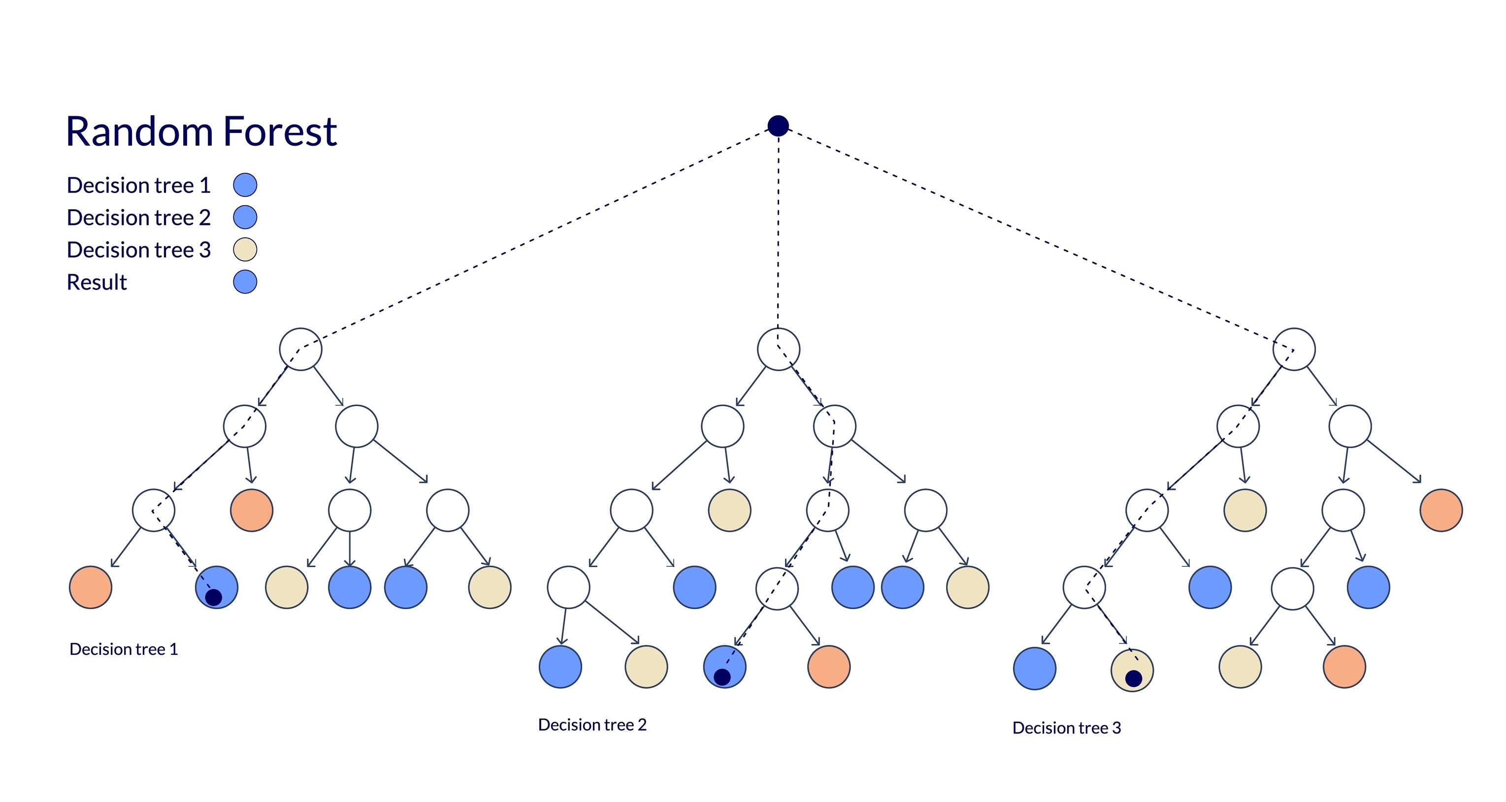
You are absolutely right. Welcome to the Random Forest.

11. Motivation: The Wisdom of Crowds

We established that a single Decision Tree is prone to overfitting. It’s like asking one highly opinionated friend for a movie recommendation. They might know your taste, but they might also be obsessed with obscure French cinema and lead you astray.

A Random Forest is the machine learning equivalent of asking 100 friends for a recommendation and going with the majority vote. While one friend might be biased or wrong, the “wisdom of the crowd” usually converges on the correct answer.

By combining many individual trees, we create a model that is more robust, stable, and accurate than any single constituent tree.

12. Ensemble, Bagging, and The Bias/Variance Trade-off

Random Forest is an Ensemble technique, meaning it combines multiple models to produce a single prediction. Specifically, it relies on a concept called Bagging.

What is Bagging?

Bagging stands for Bootstrap Aggregating. It involves two steps:

1. Bootstrapping: Creating many random subsets of the training data (sampling with replacement).
2. Aggregating: Training a separate model on each subset and combining their predictions.

The Math of Bias and Variance

• Single Decision Tree: Has Low Bias (it can model complex patterns) but High Variance (it changes drastically with small data changes).
• Random Forest: Maintains the Low Bias of the individual trees but significantly Reduces Variance.

Mathematically, if you have $B$ independent random variables (trees) each with variance $\sigma^2$, the variance of their average is $\frac{\sigma^2}{B}$.

While trees in a forest aren’t perfectly independent (they are trained on similar data), the randomization attempts to decorrelate them as much as possible, driving the variance down.

13. The Training Algorithm: Controlling the Chaos

A Random Forest is not just “Bagging trees.” It adds a second layer of randomness to ensure the trees are diverse. If we just bagged trees, they would all likely split on the strongest feature (e.g., “Lead Actor”) at the root, making them highly correlated.

To fix this, Random Forest modifies the tree-growing algorithm:

The Algorithm

Given a training set $D$ with $N$ samples and $P$ features, and a desired number of trees $B$:

For $b = 1$ to $B$:

1. Bootstrap Sample: Draw a sample $D_b$ of size $N$ from $D$ with replacement.
2. Grow Tree $T_b$: Grow a decision tree on $D_b$. However, at each node split:
   • Do not look at all $P$ features.
   • Select a random subset of $m$ features, where $m < P$.
   • Find the best split only among these $m$ features.
   • Split the node.
   • Repeat until the tree is fully grown (no pruning is usually applied).

Choosing $m$ (Max Features)

The bounding of features is the “secret sauce.” Common defaults are:

• Classification: $m \approx \sqrt{P}$
• Regression: $m \approx P/3$

14. Inference: Making Predictions

Once we have trained our forest of trees ${T_1, T_2, …, T_B}$, inference is simply an aggregation process. Let $x$ be a new input vector (a new movie).

For Regression

We take the average of the predictions from all individual trees.

\[\hat{y} = \frac{1}{B} \sum_{b=1}^{B} T_b(x)\]

For Classification

We can use “Hard Voting” or “Soft Voting.”

• Hard Voting (Majority Vote): Let $C_b(x)$ be the class predicted by tree $b$.

  \[\hat{y} = \text{mode} \{ C_1(x), C_2(x), ..., C_B(x) \}\]

• Soft Voting (Averaged Probabilities): This is generally preferred. Let $p_b(c \vert x)$ be the probability that tree $b$ assigns to class $c$. We average the probabilities across all trees and pick the class with the highest average.

  \[\hat{y} = \operatorname*{argmax}_c \left( \frac{1}{B} \sum_{b=1}^{B} p_b(c|x) \right)\]

15. Bootstrapping and Out-of-Bag (OOB) Score

When we create a bootstrap sample of size $N$ from a dataset of size $N$ with replacement, statistically, about 36.8% of the unique rows are left out.

The Setup: Imagine a dataset with $N$ rows. To create a bootstrap sample for one tree, we draw $N$ times from this dataset with replacement.

1. Probability of being picked: The probability of picking a specific row (let’s call it Row $i$) in a single draw is $\frac{1}{N}$.
2. Probability of NOT being picked: Conversely, the probability of not picking Row $i$ in a single draw is $1 - \frac{1}{N}$.
3. Probability of NOT being picked in $N$ draws: Since the draws are independent, we multiply the probability $N$ times: \(P(\text{Row } i \text{ is OOB}) = \left(1 - \frac{1}{N}\right)^N\)

The Limit: We want to know what this probability approaches as our dataset size ($N$) grows large. This brings us to a fundamental limit in calculus related to Euler’s number ($e$).

Recall the definition of $e$:

\[\lim_{N \to \infty} \left(1 + \frac{1}{N}\right)^N = e \approx 2.718\]

Our equation is slightly different (it has a minus sign), which converges to the inverse of $e$:

\[\lim_{N \to \infty} \left(1 - \frac{1}{N}\right)^N = \frac{1}{e} \approx \frac{1}{2.718} \approx \mathbf{0.368}\]

These left-out rows are called Out-of-Bag (OOB) samples.

This gives us a superpower: Built-in Validation. For every specific row in our dataset, there are several trees in the forest that never saw that row during training. We can push that row down only those specific trees to get a prediction.

The OOB Score is the aggregated accuracy (or $R^2$) of these predictions. It acts as a proxy for cross-validation without the need to explicitly set aside a test set.

16. Feature Importance via OOB (Permutation Importance)

While we can use Gini-based importance (summing gain across splits), Random Forests allow for a more robust method using OOB data, called Permutation Importance.

The logic is simple: If a feature is important, shuffling its values should break the model’s predictions.

The Algorithm:

1. Calculate the baseline OOB accuracy of the forest.
2. For a specific feature $j$ (e.g., “Lead Actor”):
   • Randomly shuffle the values of column $j$ in the OOB data (breaking the relationship between the feature and the target).
   • Re-calculate the OOB accuracy with this “broken” data.
3. Importance of Feature $j$ = (Baseline Accuracy) - (Shuffled Accuracy).

If the accuracy drops significantly, the feature is important. If it stays the same (or improves), the feature was useless (or noise).

Let’s illustrate how we calculate feature importance using the “Permutation” method on OOB data.

The Scenario: We have a trained Random Forest. We are looking at Tree #1. Tree #1 has an OOB set of 4 movies. The tree correctly predicts all of them based on the “Lead Actor” (Actual Signal) and ignores “Day of Week” (Noise).

Baseline Performance:

• OOB Data:
  1. [Hanks, Monday] -> Watched (Tree Predicts: Watched) ✅
  2. [Hanks, Friday] -> Watched (Tree Predicts: Watched) ✅
  3. [Pitt, Tuesday] -> Skip (Tree Predicts: Skip) ✅
  4. [Pitt, Friday] -> Skip (Tree Predicts: Skip) ✅
• Baseline Accuracy: 4/4 = 100%

Test 1: Check Importance of “Lead Actor” We shuffle the “Lead Actor” column randomly in the OOB data. The “Day of Week” stays the same.

• Shuffled Data:
  1. [Pitt, Monday] -> Truth is Watched. Tree sees Pitt, Predicts: Skip. ❌
  2. [Hanks, Friday] -> Truth is Watched. Tree sees Hanks, Predicts: Watched. ✅
  3. [Hanks, Tuesday] -> Truth is Skip. Tree sees Hanks, Predicts: Watched. ❌
  4. [Pitt, Friday] -> Truth is Skip. Tree sees Pitt, Predicts: Skip. ✅
• New Accuracy: 2/4 = 50%
• Importance Score: $100\% - 50\% = \mathbf{50\%}$ (Huge Drop = High Importance)

Test 2: Check Importance of “Day of Week” We reset the data and this time shuffle the “Day of Week” column.

• Shuffled Data:
  1. [Hanks, Friday] -> Truth is Watched. Tree sees Hanks, Predicts: Watched. ✅
  2. [Hanks, Tuesday] -> Truth is Watched. Tree sees Hanks, Predicts: Watched. ✅
  3. [Pitt, Monday] -> Truth is Skip. Tree sees Pitt, Predicts: Skip. ✅
  4. [Pitt, Friday] -> Truth is Skip. Tree sees Pitt, Predicts: Skip. ✅
• New Accuracy: 4/4 = 100%
• Importance Score: $100\% - 100\% = \mathbf{0\%}$ (No Drop = Useless Feature)

By measuring how much the model “panics” when a feature is broken, we learn how heavily it relied on it.

17. Decision Tree vs. Random Forest: The Showdown

To wrap up, how do you choose between the simplicity of a single tree and the power of a forest? Here is the cheat sheet.

Feature	Decision Tree 🌳	Random Forest 🌲🌲🌲
Interpretability	High. You can visualize the exact rules (White Box). Great for explaining “Why” to stakeholders.	Low. It is a “Black Box” of hundreds of trees. You get feature importance, but not exact decision paths.
Performance	Lower. Prone to high variance and errors on unseen data.	High. Generally achieves state-of-the-art accuracy for tabular data.
Overfitting	High Risk. Will memorize noise if not pruned heavily.	Low Risk. Averaging many trees cancels out the noise and bias errors.
Training Speed	Fast. Building one tree is computationally cheap.	Slower. Building 100+ trees takes time (though it can be parallelized).
Inference Speed	Ultra Fast. Just a few if-else statements.	Slower. The data must pass through every tree in the forest.
Data Requirements	Requires careful preprocessing (pruning parameters).	Works well “out of the box” with default settings. Handles outliers well.
Decision Boundary	Orthogonal (step-wise) and often jagged.	Smoother and more stable boundaries due to averaging.
Best Used For…	Rapid prototyping, simple baselines, and when explainability is the top priority.	Kaggle competitions, high-stakes predictions, and when accuracy is the top priority.