Packing Intelligence into Fewer Bits: Non-Linear Quantization in LLMs
A 70-billion-parameter LLM stored in 16-bit floats needs roughly 140 GB of memory, more than most GPUs can hold. Quantization shrinks the model by replacing those 16-bit floats with much smaller integers (4-bit, for example), cutting memory by $4\times$.
The simplest approach is linear quantization, which spaces the quantized values evenly across the weight range, like the markings on a ruler. We covered the full mechanics of linear quantization in our previous post, including affine mapping, symmetric vs. asymmetric variants, and how they map to hardware. If you haven’t read it yet, it’s a worthwhile primer before diving in here.
Linear quantization works, but it has a serious blind spot: LLM weights are not evenly spread. They usually follow a bell curve, heavily clumped around zero, with only a handful of outliers far from the center.
When a uniform ruler meets a bell-curve distribution, the result is wasted precision exactly where it matters most. This post walks through that problem step by step and then explores three progressively smarter solutions:
- Quantile Quantization — match bins to where the data actually lives.
- NormalFloat4 (NF4) — pre-compute optimal bins once, skip expensive sorting.
- Clustering-Based Quantization — let k-means custom-tailor the bins to any distribution.
We will wrap up with a brief look at GPTQ and AWQ, two popular production methods that take a different approach entirely, with a dedicated deep dive coming in a future post.
1. Linear Quantization and Its Limits
How Symmetric Linear Quantization Works
In symmetric linear quantization, we build a grid that is perfectly symmetric around zero, the natural center of LLM weight distributions. The entire grid is controlled by a single number: the scale factor $s$.
Here is the recipe. Given a weight matrix, find the largest absolute value, $\alpha = \max(\lvert w_i \rvert)$. Then:
1
s  =  α / (2^(b-1) - 1)
For 4-bit quantization, $2^{b-1} - 1 = 7$, so integer codes run from $-7$ to $+7$, that is 15 distinct levels. Every weight gets encoded and later reconstructed as:
1
2
q  =  clamp(round(w / s), -7, +7)     ← quantize   (store this integer)
ŵ  =  q × s                           ← dequantize (use this float at inference)
Why 15 levels and not 16? A 4-bit integer can represent 16 values (say, $-8$ to $+7$). But symmetric quantization deliberately drops one code to keep the grid perfectly balanced around zero. That guarantees the exact float value
0.0is always representable — an important property for neural networks where zero means “no connection.”
Anatomy of a Bin: Boundaries, Centers, and Codes
Let’s make this concrete. Suppose the largest weight in our matrix is $\alpha = 2.0$. Then:
1
s  =  2.0 / 7  ≈  0.286
Every integer code q lives at the center of a bin in float space. The boundaries between adjacent bins fall at half-integer multiples of s:
1
2
3
4
5
6
7
8
Boundaries are denoted by B:
         B          B         B          B          B
         ↓     ⋮    ↓     ⋮    ↓     ⋮    ↓     ⋮    ↓
─────────|─────⋮────|─────⋮────|─────⋮────|─────⋮────|─────────
      -0.429   ⋮ −0.143   ⋮  0.143   ⋮  0.429   ⋮  0.714
               ⋮          ⋮          ⋮          ⋮
centers:    −0.286      0.000      0.286      0.571
             q=−1        q=0        q=1        q=2
Here is the breakdown for a few representative bins:
| Code $q$ | Bin center $q \cdot s$ | Lower boundary $(q - \frac{1}{2}) \cdot s$ | Upper boundary $(q + \frac{1}{2}) \cdot s$ | Bin width |
|---|---|---|---|---|
| $-7$ | $-2.000$ | $-2.000$ (clamped at $-\alpha$) | $-1.857$ | $s/2$ |
| $-1$ | $-0.286$ | $-0.429$ | $-0.143$ | $s$ |
| $0$ | $0.000$ | $-0.143$ | $+0.143$ | $s$ |
| $1$ | $+0.286$ | $+0.143$ | $+0.429$ | $s$ |
| $7$ | $+2.000$ | $+1.857$ | $+2.000$ (clamped at $+\alpha$) | $s/2$ |
A few things to notice:
- Integer codes sit at bin centers, not boundaries. The multiples of $s$ ($0.000$, $\pm 0.286$, $\pm 0.571$, …) are the points where each code lives. The boundaries are halfway between those points.
- Zero is a bin center, not a fence. $q = 0$ owns the region $(-0.143, +0.143)$. This gives us 7 negative bins + 1 zero bin + 7 positive bins = 15 bins total.
- Edge bins are half-width. The bin for $q = +7$ only spans from $1.857$ to $2.000$ (width $= s/2$), because $\alpha = 7s$ sits exactly at the outer limit. The dequantized value ($2.000$) lands at the edge of this truncated bin, not its midpoint — a small but real source of bias for the most extreme weights.
What Happens Inside a Single Bin
Here is the crucial consequence: every weight that falls inside the same bin gets the exact same dequantized value. The individual float is gone forever.
Take $q = 1$, which covers the range $(0.143, 0.429)$ and reconstructs everything to $0.286$:
| Original weight $w$ | $\text{round}(w / 0.286)$ | Stored code $q$ | Dequantized $\hat{w}$ | Error $w - \hat{w}$ |
|---|---|---|---|---|
| $0.150$ | round(0.525) | $1$ | $0.286$ | $-0.136$ |
| $0.200$ | round(0.700) | $1$ | $0.286$ | $-0.086$ |
| $0.286$ | round(1.000) | $1$ | $0.286$ | $0.000$ |
| $0.350$ | round(1.225) | $1$ | $0.286$ | $+0.064$ |
| $0.420$ | round(1.470) | $1$ | $0.286$ | $+0.134$ |
Five completely different weights, and the model sees all of them as $0.286$ at inference time. The error is zero only for the weight that happened to sit at exactly the bin center. Everyone else loses precision, up to a worst-case error of $s/2 \approx 0.143$ right at the bin edges.
Wasted Bins on a Bell Curve
Now imagine applying this grid to actual LLM weights. Suppose our weight matrix contains 2,000 values drawn from a typical distribution: $\text{Normal}(\mu = 0, \sigma = 0.35)$.
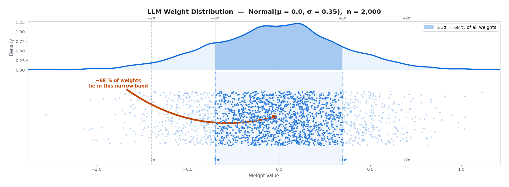
The top panel shows the density curve (the KDE), the bottom shows every weight as an individual dot. Notice how densely the dots pack inside the darker $\pm 1\sigma$ band (~68% of all weights) and how quickly they thin out in the tails. Any quantization scheme has to grapple with this reality.
The linear quantizer does not care where the weights live. It divides the full range: say $-1.10$ to $+1.07$, into equal slices. Here is what actually happens:
| Bin region | Distance from zero | Approx. weights | Share of total |
|---|---|---|---|
| Outermost 4 bins (2 each side) | beyond $\pm 2\sigma$ | ~100 combined | ~5% |
| Next 4 bins (2 each side) | $\pm 1\sigma$ - $\pm 2\sigma$ | ~540 combined | ~27% |
| Central bins | within $\pm 1\sigma$ | ~1,360 combined | ~68% |
The central bins are fighting over 68% of all weights, while the outermost bins collectively hold fewer than 100 values. Those edge bins consume a large share of the bit-budget while contributing almost nothing.
Why Overcrowded Bins Destroy Model Quality
The numbers above tell us how many weights land in each bin. Let’s now see why that matters for the model’s accuracy.
With $\alpha = 1.05$ and 4-bit symmetric quantization:
1
s = 1.05 / 7 = 0.150
Bin $q = 0$ covers $(-0.075, +0.075)$. A weight at $w = 0.012$ and a weight at $w = 0.071$ both round to $q = 0$ and both reconstruct as $\hat{w} = 0.000$. Their difference of $0.059$, which may encode a distinct learned feature — is permanently erased. The model cannot tell them apart.
The worst-case error per weight is $s/2 = 0.075$. That sounds small on its own, but consider this: in a 512-dimensional dot product where every weight carries up to $\pm 0.075$ error, the accumulated output deviation can reach $0.075 \times 512 \approx 38$, large enough to meaningfully distort downstream activations.
The outlier amplification problem. Because $s$ is anchored to the single largest weight, one rogue outlier inflates the scale for the entire matrix:
1
2
Without outlier:   s = 1.05 / 7 = 0.150   →  bin 0 covers (-0.075, +0.075)
With one outlier:  s = 2.10 / 7 = 0.300   →  bin 0 covers (-0.150, +0.150)
| Bins | Float range | % of weights collapsed here |
|---|---|---|
| $q = 0$ | $(-0.150, +0.150)$ | ~33% $\to$ all map to $0.000$ |
| $q = \pm 1$ | $(0.150, 0.450)$ and mirror | ~47% $\to$ all map to $\pm 0.300$ |
| Central 3 bins total | ~80% |
Because our weights are distributed as $\mathcal{N}(0, 0.35)$, the probability of landing in the symmetric interval $[-x, +x]$ is $2\Phi(x/0.35) - 1$, where $\Phi$ is the standard-normal CDF. For bin $q = 0$ that gives $2\Phi(0.429) - 1 \approx 33\%$, and for bin $q = \pm 1$ it gives $2[\Phi(1.286) - \Phi(0.429)] \approx 47\%$.
One outlier has hijacked the grid. ~80% of 2,000 weights are now represented by just three float values ($-0.300$, $0.000$, $+0.300$), up from ~48% without the outlier.
Where does that ~48% baseline come from? Without the outlier, $s = 0.150$. So bin $q = 0$ is half as wide — spanning $(-0.075, +0.075)$, and bin $q = \pm 1$ spans $(0.075, 0.225)$ on each side. Applying the same $2\Phi(x/0.35) - 1$ formula:
| Bins | Float range | Share of weights |
|---|---|---|
| $q = 0$ | $(-0.075, +0.075)$ | $2\Phi(0.214) - 1 \approx 17\%$ |
| $q = \pm 1$ | $(0.075, 0.225)$ and mirror | $2[\Phi(0.643) - \Phi(0.214)] \approx 31\%$ |
| Central 3 bins total | ~48% |
So the scale factor doubling (from $0.150$ to $0.300$) lifts the central-three-bin collapse from ~48% to ~80%, a 32-point jump triggered by one outlier.
This is the fundamental asymmetry: the weights that matter most — the dense center, where subtle differences encode learned representations, bear the full cost of a scale factor set by the rarest values in the distribution.
Linear Quantization in Action
Now let’s apply linear quantization to the same 2,000 weights and colour each dot by the bin it was assigned to:
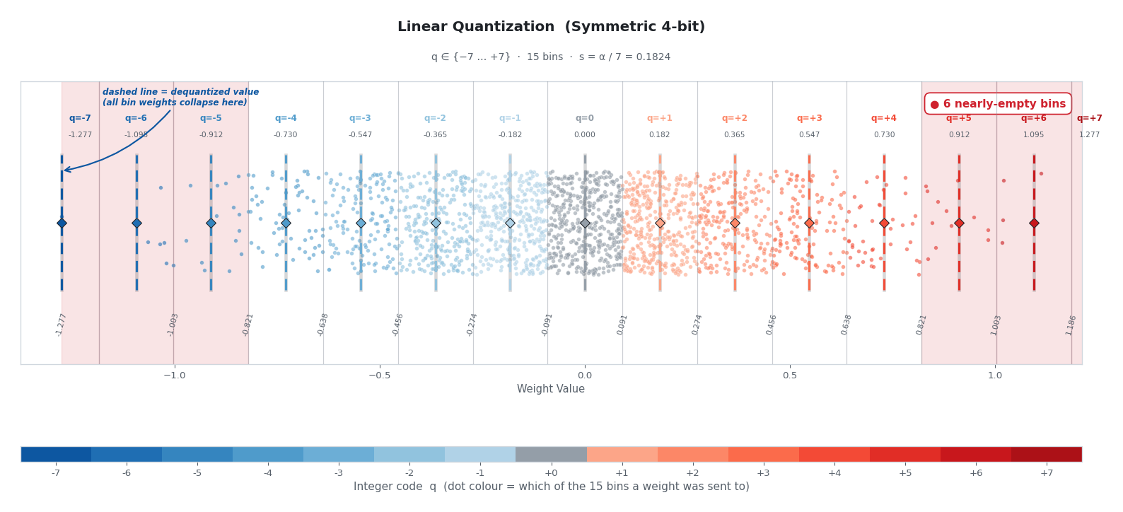
A few things jump out. Nearly all the dots collapse into the same handful of colours near the centre, while the red-shaded outer bins — each still consuming a full 4-bit code sit almost empty. The dashed vertical lines mark each bin’s reconstruction target. Every weight inside a bin gets collapsed to that single float value. Reconstruction precision where the data actually lives is wrecked, reconstruction precision where no data lives is wasted.
2. Quantile Quantization: The First Fix
The Key Question: Equal Counts, Not Equal Widths
Instead of asking “how wide should each bin be?”, quantile quantization asks a different question:
“Where should I draw boundaries so that every bin holds the same number of weights?”
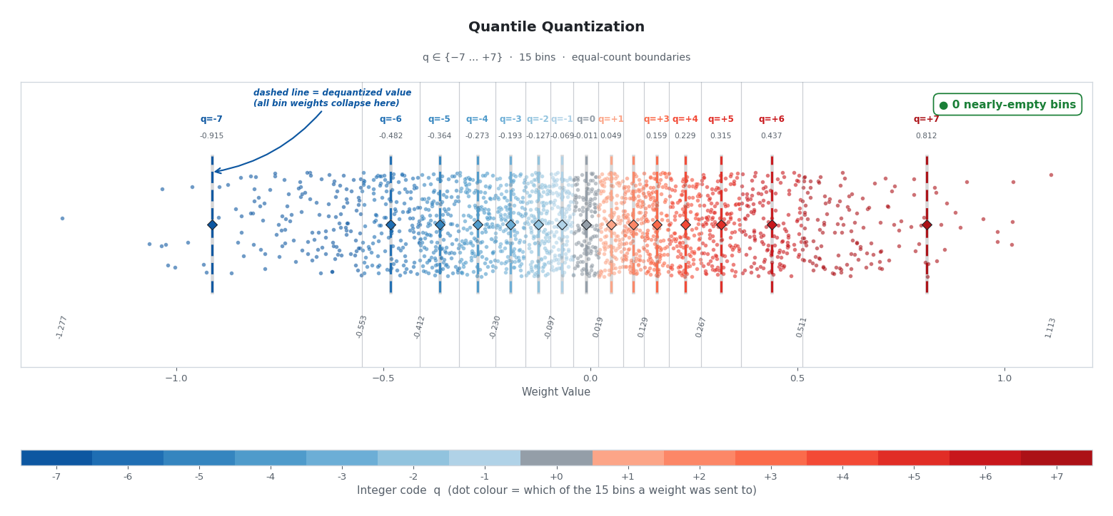
The vertical cuts above are packed tightly near zero, where the data is dense, and stretched far apart at the tails. Moving just a tiny step along the x-axis near zero is enough to fill a bin with its share of weights. At the tails, it takes a huge step to find enough outliers to fill one.
The result: High precision exactly where the model needs it (the dense center) and gracefully relaxed precision at the sparse tails without spending a single extra bit.
Computing the Boundaries with Percentiles
For 15 bins (symmetric 4-bit), we need 16 boundary points. We simply find the percentile values that split the weight distribution into 15 equal-count groups:
1
2
3
import numpy as np

bin_edges = np.percentile(weights, np.linspace(0, 100, 16))
Under the hood, np.percentile with np.linspace(0, 100, 16) finds the 0th, 6.67th, 13.33th, … 93.33th, and 100th percentiles. Each of the 15 intervals between consecutive edges holds exactly $\frac{1}{15}$ th of the data.
The outcome is exactly what the image above shows: the quantized integer assignments are now uniformly distributed across all bins. No wasted codes, no overcrowded bins — every bin earns its keep.
The Sorting Bottleneck
Finding exact percentiles requires sorting the data — an $O(N \log N)$ operation. When you are quantizing an LLM with 70 billion weights, sorting every block during training or inference is painfully slow.
This bottleneck is what leads us to our next method.
3. NormalFloat4 (NF4): The Precomputed Shortcut
The Insight: Skip the Sort
Think back to the bell curve we laid over our data. If we know ahead of time that LLM weights almost always follow a normal distribution, we can figure out where the percentile boundaries should go without ever sorting the actual weights.
The trick: Instead of looking at the data, look at the theoretical standard normal distribution ($\mu = 0$, $\sigma = 1$). Using a statistical tool called the Inverse CDF, we can instantly compute the exact Z-scores where the area under the curve hits 6.67%, 13.33%, and so on — no data required.
The Inverse CDF: Our Key Mathematical Tool
Before building the NF4 grid, it is worth spending a moment on the mathematical idea that makes it all possible.
The Cumulative Distribution Function (CDF) of a probability distribution, written $\Phi(x)$ for the standard normal, answers one simple question: “What fraction of the data falls at or below value $x$?”
\[\Phi(0) = 0.5, \qquad \Phi(1) = 0.841, \qquad \Phi(-1) = 0.159\]So if our weights follow a standard normal distribution, exactly half of them fall below zero, about 84% fall below $+1$, and so on.
The Inverse CDF (or quantile function) $\Phi^{-1}(p)$ flips the question: “What value $x$ has exactly $p$ fraction of the data below it?”
\[\Phi^{-1}(0.5) = 0, \qquad \Phi^{-1}(0.841) = 1, \qquad \Phi^{-1}(0.159) = -1\]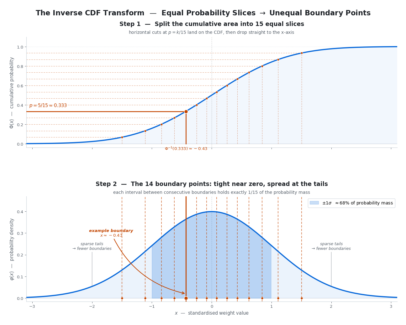
Here is why this matters. If we want to split a standard normal distribution into 15 equal-probability bins, we need boundary points at every $\frac{1}{15}$ th of the cumulative area: the 6.67th, 13.33th, …, 93.33th percentiles. Each of those boundary points is simply one evaluation of $\Phi^{-1}$:
\[\text{boundary}_k = \Phi^{-1}\!\left(\frac{k}{15}\right), \quad k = 1, 2, \dots, 14\]The beautiful part: for a known distribution, these values are fixed constants that can be computed once, offline, before ever seeing the model’s weights. No sorting, no data — just a well-known statistical function evaluated 14 times. NF4 is built entirely on this insight.
Phase 1: Building the NF4 Grid (Offline)
Let $\Phi^{-1}(p)$ be the inverse CDF of the standard normal distribution — the function that returns the Z-score for a given cumulative probability $p$.
For $k$-bit quantization ($k = 4$, so $2^k = 16$ values), we calculate 16 theoretical grid points:
\[v_i = \Phi^{-1}\!\left(\frac{i + 0.5}{2^k}\right) \quad \text{for } i = 0, 1, \dots, 15\](The actual QLoRA paper uses a slightly more complex asymmetric split to guarantee that $0.0$ is one of the representable values, but the inverse-CDF principle is the same.)
Wait — didn’t we use 14 boundaries for 15 bins earlier? Why 16 grid points now?
The two sections compute different things:
- Boundaries ($\Phi^{-1}(k/15)$, for $k = 1, \dots, 14$) are the cuts between bins. Fifteen bins need fourteen interior cuts, which is why we had 14 boundary points — matching the symmetric 4-bit encoding that drops one of the 16 codes to keep $0.0$ perfectly centred.
- Grid points ($v_i$) are the reconstruction targets — the single float each bin dequantizes back to. NF4 uses all $2^4 = 16$ codes with no symmetry constraint, so we store 16 of them.
The $(i + 0.5)/2^k$ in the formula lands each grid point at the midpoint (in probability mass) of its equal-probability slice — the “typical” value for any weight that falls there.
These Z-scores extend beyond $\pm 1$, so we normalize them to fit within $[-1, 1]$:
\[q_i = \frac{v_i}{\max(|v|)}\]Plugging the formula through for 4-bit gives:
| $i$ | $(i + 0.5)/16$ | $v_i = \Phi^{-1}(\cdot)$ | $q_i = v_i / 1.863$ |
|---|---|---|---|
| $0$ | $0.0313$ | $-1.863$ | $-1.000$ |
| $1$ | $0.0938$ | $-1.318$ | $-0.708$ |
| $2$ | $0.1563$ | $-1.010$ | $-0.542$ |
| $3$ | $0.2188$ | $-0.776$ | $-0.417$ |
| $4$ | $0.2813$ | $-0.579$ | $-0.311$ |
| $5$ | $0.3438$ | $-0.402$ | $-0.216$ |
| $6$ | $0.4063$ | $-0.237$ | $-0.127$ |
| $7$ | $0.4688$ | $-0.078$ | $-0.042$ |
| $8$ | $0.5313$ | $+0.078$ | $+0.042$ |
| $9$ | $0.5938$ | $+0.237$ | $+0.127$ |
| $10$ | $0.6563$ | $+0.402$ | $+0.216$ |
| $11$ | $0.7188$ | $+0.579$ | $+0.311$ |
| $12$ | $0.7813$ | $+0.776$ | $+0.417$ |
| $13$ | $0.8438$ | $+1.010$ | $+0.542$ |
| $14$ | $0.9063$ | $+1.318$ | $+0.708$ |
| $15$ | $0.9688$ | $+1.863$ | $+1.000$ |
The plot below drops all 16 grid points onto the standard-normal curve they were carved out of — each diamond sits at its $v_i$ along the Z-axis, and the dashed line above it climbs to the density $\varphi(v_i)$.
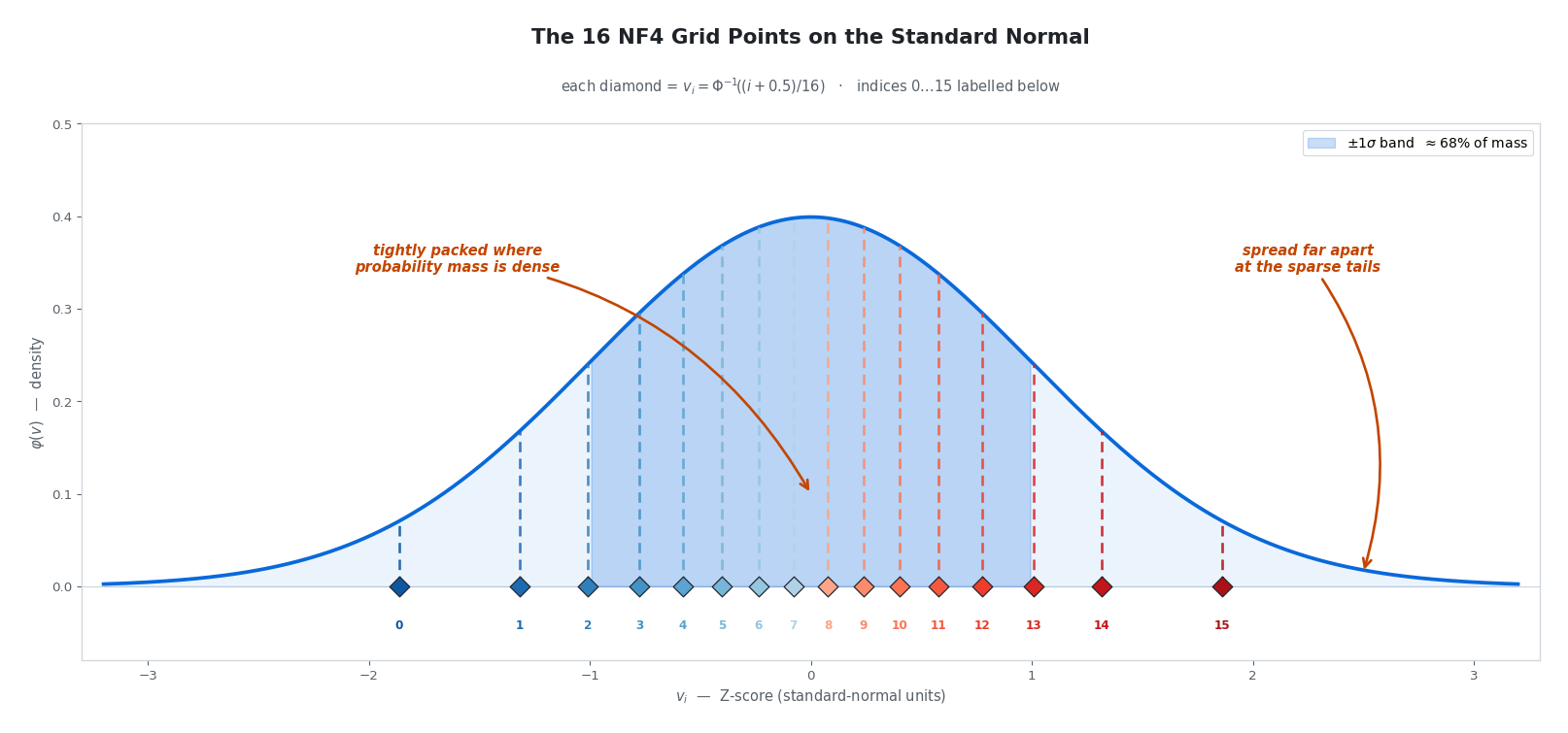
Look at the spacing in the rightmost column of the table (or equivalently, at the horizontal gaps between diamonds in the figure): grid points are packed tightly near zero (adjacent values differ by only $\sim 0.085$ between $q_7$ and $q_8$) and stretched far apart at the tails ($\sim 0.29$ between $q_{14}$ and $q_{15}$). This is precisely the “more precision where the data is dense” pattern we wanted — now baked into 16 numbers we compute once and never touch again.
This fixed array $q = {-1.000, -0.708, \dots, +0.708, +1.000}$ lives permanently in GPU memory as a simple lookup table.
(Note: this symmetric version has no exact $q = 0$, the two closest points are $\pm 0.042$. QLoRA’s real NF4 uses an asymmetric eight-negative / seven-positive split plus a forced $0.0$, so inert weights map exactly to zero. The inverse-CDF principle is identical; only the exact numbers shift by a hair.)
Phase 2: Block-wise Quantization (Compression)
Now we bring in the actual weights. To protect against outliers, NF4 uses block-wise quantization: instead of normalizing a whole layer at once, it chops the weights into small, independent blocks (typically 64 weights per block).
For each block $\mathbf{w} = {w_1, w_2, \dots, w_{64}}$:
Step 1 — Find the block’s scale factor:
\[c = \max_{j} |w_j|\]Step 2 — Normalize and map to the nearest grid point:
Divide each weight by $c$ to squeeze it into $[-1, 1]$, then find the index of the closest value in the NF4 grid:
\[I_j = \arg\min_{i \in \{0 \dots 15\}} \left| \frac{w_j}{c} - q_i \right|\]What gets stored: For each weight, we keep only the 4-bit integer $I_j$. For each block, we save one 16-bit float scale factor $c$.
Why blocks matter: a toy example
Imagine 64 weights — 63 are tightly packed near zero, but weight #45 is a massive outlier at 2.5.
- Global scaling: We divide everything by 2.5. The 63 good weights get crushed into a narrow strip near zero. Nearly all of them fall into just one or two bins. Precision destroyed.
- Block-wise scaling (block size = 32): Block 1 (no outlier, max = 0.19) gets divided by 0.19 — the weights spread beautifully across the full grid. Block 2 (has the outlier, max = 2.5) gets compressed, but the damage is quarantined. The other 32 weights in Block 1 are completely unaffected.
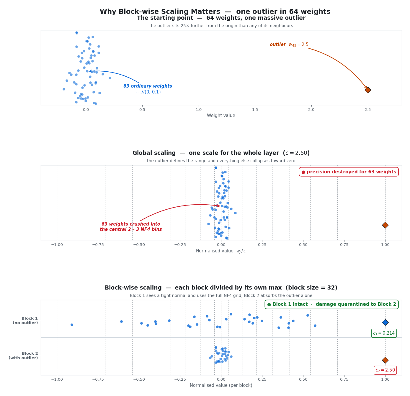
The figure above makes the trade-off concrete. The top panel shows the raw weights — 63 ordinary samples and the lone outlier sitting 25× further out. The middle panel applies one global scale factor ($c = 2.5$): the outlier defines the range and every other weight collapses into the central two or three NF4 bins. The bottom panel splits the same weights into two blocks of 32, Block 1 (whose own max is just 0.19) now spreads beautifully across the full $[-1, +1]$ grid, while the damage from the outlier stays confined to Block 2 — and even there, only 31 of the 64 weights pay the cost instead of all 63.
Why Absolute Max Scaling, Not Standardization?
You might wonder: why not subtract the mean and divide by the standard deviation? After all, that is the textbook way to normalize data to a standard normal. Three practical reasons:
- The zero-point problem (the biggest reason). In neural networks,
0.0is a special value. It means “no connection” and lets hardware skip entire multiplications. Subtracting the mean shifts0.0to some awkward float like $-0.014$. Absolute max scaling guarantees that0.0stays exactly0.0. - Redundant math. Thanks to LayerNorm and RMSNorm used during training, LLM weights already hover around a mean of virtually zero. Subtracting the mean is wasted compute.
- Storage overhead. Standardization requires storing two FP16 values per block ($\mu$ and $\sigma$). Max scaling stores just one ($c$). Over billions of parameters, that extra overhead eats into the memory savings we are trying to achieve.
Phase 3: Dequantization with a Lookup Table
When the GPU needs the weights for inference, the reversal is elegantly simple. For a stored 4-bit integer $I_j$ and block scale $c$:
\[\hat{w}_j = c \cdot q_{I_j}\]The GPU reads integer 14, jumps to slot 14 in its cached lookup table, grabs the float (say $0.723$), and multiplies by the block’s scale ($0.15$) to get $0.723 \times 0.15 = 0.109$. That is it — one memory fetch, one multiplication.
“Fake” 4-Bit: Why Memory Bandwidth Is the Real Win
There is a crucial nuance that trips up a lot of people: NF4 does not do math in 4-bit. The dequantization happens on the fly inside the GPU’s registers, milliseconds before the actual computation. Once the weight is reconstructed back into a 16-bit float, the GPU multiplies it by the incoming activations using standard FP16 or BF16 arithmetic.
So if the math still happens in 16-bit, why bother? Because the real bottleneck in LLMs is not compute speed — it is memory bandwidth. Moving data from VRAM into the GPU’s processing cores is the slowest part of the pipeline. By storing weights as 4-bit integers, we shove $4\times$ as many weights through the memory bus per cycle. The result: dramatically faster inference and the ability to fit massive models on a single GPU.
4. Clustering-Based Quantization: The Custom Tailor
When the Bell Curve Does Not Fit
NF4 is brilliant, but it has a blind spot: it strictly assumes the weights follow a symmetrical bell curve. What if a specific layer has a bimodal distribution (two distinct clumps)? Or what if it is heavily skewed to one side? The pre-calculated NF4 grid would force those weights into poorly fitting bins.
Clustering-based quantization (often using the k-means algorithm) throws away all distributional assumptions. Instead of a theoretical curve, it looks at the actual data and custom-builds a unique codebook for every block of weights.
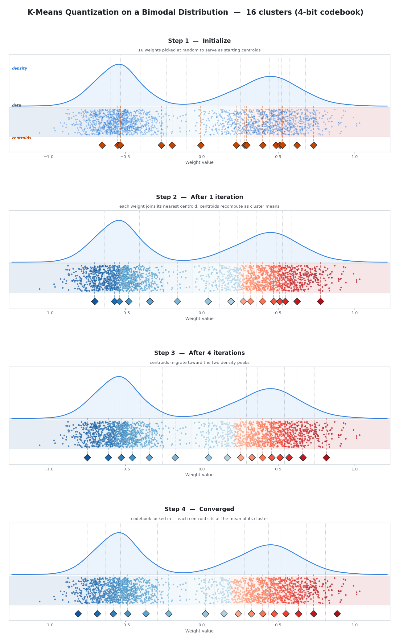
The K-Means Process
For 4-bit quantization, we need 16 clusters. Here is how the algorithm finds them:
- Initialize. Pick 16 actual weight values from the block as starting centroids.
- Assign. Every weight calculates its distance to all 16 centroids and joins the team of whichever centroid is closest.
- Update. Each centroid moves to the exact mean of all weights currently assigned to it.
- Repeat. Steps 2-3 loop until the centroids stop moving and settle into their optimal positions.
The Custom Codebook
Once k-means converges, we save those 16 final centroid values as a codebook — a custom lookup table. Each original weight is replaced with a 4-bit integer (0-15) indicating which cluster it belongs to.
During inference, dequantization works exactly like NF4: the GPU reads integer 12, looks up slot 12 in the codebook, and instantly gets the float value back.
The Catch: Compute Cost
If clustering adapts so perfectly to the data, why is it not the default? Because running k-means requires iterative distance calculations across billions of parameters. For a 70B model, this takes hours. NF4 may be slightly less precise, but its boundaries are computed once and applied everywhere — essentially free.
Clustering is typically reserved for post-training quantization, where you are willing to invest significant compute to squeeze out every last drop of precision before deploying to production.
5. GPTQ and AWQ: Linear Grids, Smarter Optimization
Here is an interesting twist to end on: the most popular production quantization methods today actually use linear (uniform) grids. Modern GPU Tensor Cores are designed for lightning-fast math on uniformly spaced integers — non-linear grids require a per-weight lookup that kills throughput. So the industry has circled back to simple grids, but brought sophisticated math to bear on how weights land on them.
GPTQ takes the view that quantizing one weight introduces a small error, but you can mathematically adjust the neighboring weights in the same row to cancel it out — using the Hessian matrix to guide exactly how much correction each neighbor needs.
AWQ starts from a different observation: roughly 1% of weights are “salient” — they get multiplied by the largest activation values, so any quantization error there gets amplified the most. AWQ scales those critical weights up before quantization so they land far more accurately on the grid, then scales them back down at inference time.
Both methods produce standard 4-bit integers that Tensor Cores can crunch at full speed, with their non-linear cleverness baked in during a one-time offline compression step. We will dig into the full mechanics — the Hessian updates, the activation calibration, the head-to-head tradeoffs — in a dedicated future post.
Wrapping Up
Here is the journey we have taken, from simplest to most sophisticated:
| Method | Grid Type | Key Idea | Cost | Best For |
|---|---|---|---|---|
| Linear Symmetric | Uniform | Equal-width bins | Instant | Baseline / when speed is all that matters |
| Quantile | Non-uniform | Equal-count bins (via percentiles) | Requires sorting ($O(N \log N)$) | Theoretical foundation |
| NF4 | Non-uniform | Pre-computed quantile grid assuming normality | Instant (grid is hardcoded) | LoRA training (QLoRA) |
| K-Means Clustering | Non-uniform | Data-adaptive clusters, no assumptions | Expensive (iterative) | Post-training compression |
| GPTQ | Uniform | Error compensation via Hessian | Moderate (one pass per layer) | Production inference |
| AWQ | Uniform | Activation-aware salient-weight scaling | Moderate | Production inference |
The core lesson: there is no single best method. The right choice depends on whether you are training or serving, how much time you can spend compressing, and what hardware you are deploying to. But every method in this list starts from the same observation: LLM weights are not uniform, and respecting their distribution, whether through smarter bin placement, smarter error compensation, or smarter scaling — is the key to preserving model quality at low bit-widths.