Demystifying LLM Temperature: The Math Behind the Magic of Token Sampling

If you’ve played with any Large Language Model (LLM) API, you’ve likely tweaked the temperature slider. The conventional wisdom is simple: “Low temperature = boring and factual, High temperature = creative and chaotic.”

But as engineers and data scientists, “magic sliders” aren’t enough. What is the temperature parameter actually doing to the neural network under the hood? Does it change the model’s underlying beliefs, or just how it rolls the dice?

In this post, we’ll open the black box of LLM inference, explore the math of temperature-scaled Softmax, visualize its effect on probability distributions, and uncover a common misconception about how it interacts with Top-K and Top-P sampling.

1. The Raw Output: Logits and Softmax

Before we talk about temperature, we need to understand what an LLM actually outputs. When you feed a prompt into an LLM, the final layer doesn’t output text. It outputs a vector of raw, unnormalized numbers called logits ($z$). There is one logit for every possible token in the model’s vocabulary (which could be 50,000+ tokens).

To convert these arbitrary scores into valid probabilities (which must be between 0 and 1, and sum to 1), we pass them through the Softmax function.

Standard Softmax looks like this:

\[P(x_i) = \frac{\exp(z_i)}{\sum_j \exp(z_j)}\]

This equation translates the model’s raw confidence into a probability distribution. The token with the highest probability is the model’s “best guess” for the next word.

2. Enter the Temperature Parameter ($T$)

The temperature parameter ($T$) is simply a scaling factor injected directly into the denominator of the Softmax exponent. The Temperature-Scaled Softmax Formula:

\[P(x_i) = \frac{\exp(z_i / T)}{\sum_j \exp(z_j / T)}\]

By dividing the logits by $T$ before exponentiation, we fundamentally alter the shape of the resulting probability distribution.

The Three Regimes of Temperature

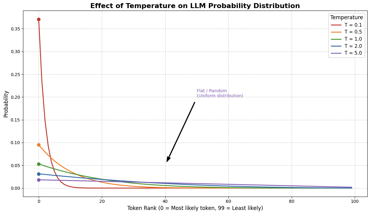
• $T = 1.0$ (The Baseline): The equation behaves as a standard Softmax. The model outputs its true, naturally calibrated confidence.

• $T \to 0$ (The Greedy Spike): Dividing by a tiny decimal is equivalent to multiplying by a huge number. This dramatically exaggerates the differences between logits. The token with the highest logit absorbs nearly 100% of the probability mass. The model becomes virtually deterministic.

• $T \to \infty$ (The Flatline): Dividing by a massive number squashes all logits close to zero. Since $e^0 = 1$, all tokens end up with roughly the same numerator. The probability distribution flattens out, approaching a perfectly uniform distribution where every word in the dictionary is equally likely.

3. The Great Misconception: Does Temperature Change the Candidate Pool?

Here is where many practitioners get confused. If temperature flattens the curve, does it change the ranking of the tokens? Does it change which tokens the downstream samplers (Top-K or Top-P) are allowed to look at?

The short answer: It preserves the rank, but its effect on the candidate pool depends entirely on your sampling strategy.

Because the exponential function is strictly monotonically increasing, dividing by a positive constant ($T$) never changes the relative ranking of the tokens. If “Apple” had a higher logit than “Banana”, “Apple” will always have a higher probability than “Banana”, at any temperature.

However, how this affects the candidate pool diverges based on your sampling algorithm:

Scenario A: Top-K Sampling

In Top-K sampling, we isolate the $K$ tokens with the highest probabilities and ignore the rest.

• Does the pool change? NO.
• Because the rank order is preserved, the exact same $K$ tokens will make up the candidate pool whether $T=0.1$ or $T=100$. Temperature dictates how the probability is distributed among those K tokens, but it doesn’t invite any new tokens to the party.

Scenario B: Top-P (Nucleus) Sampling

In Top-P sampling, we sort tokens by rank and include them in the pool until their cumulative probability reaches $P$ (e.g., $P = 0.90$).

• Does the pool change? YES, drastically.
• At $T=0.1$, the top token might hold 95% of the probability mass. The algorithm hits the 90% threshold immediately, resulting in a pool size of exactly 1 token.
• At $T=5.0$, the distribution is flat. The top token might only hold 2%. To reach the 90% cumulative threshold, the algorithm might have to scoop up the top 5,000 tokens.
• Takeaway: High temperature actively forces Nucleus Sampling to consider a vastly larger vocabulary.

4. The Final Roll of the Dice: Next Token Prediction

Once the sampling algorithm (Top-K or Top-P) has isolated the candidate pool and re-normalized their probabilities to sum to 1, the final step is random sampling. The model rolls a weighted polyhedral die to pick the winning token.

This is where the true impact of temperature is felt in the generation:

• Low Temperature: The Top-1 token might have a 99% weight in the pool. The random sampler will pick it almost every time, leading to highly predictable, repetitive, but factually grounded text.
• High Temperature: The weights inside the pool are heavily leveled. If “Apple”, “Banana”, and “Cherry” now hold 34%, 33%, and 33% respectively, the random sampler is equally likely to pick any of them. The model takes “risks,” choosing suboptimal tokens that lead the text down creative, surprising, or sometimes hallucinated paths.

Conclusion

Temperature doesn’t make an LLM “smarter” or “dumber.” It is simply a mathematical distortion applied to the model’s internal confidence before the dice are rolled.

By understanding the interplay between the Temperature-scaled Softmax and downstream algorithms like Top-P, you can move beyond randomly sliding values until the text looks good, and start engineering your generation pipelines with deterministic precision.

Appendix: Code for the visualization

import numpy as np
import matplotlib.pyplot as plt

def softmax_with_temperature(logits, temperature):
    """
    Applies temperature scaling to logits and computes the softmax probabilities.
    """
    # Prevent division by zero
    temperature = max(temperature, 1e-5)
    
    # Scale logits by temperature
    scaled_logits = logits / temperature
    
    # Subtract max for numerical stability before exponentiation
    # (This doesn't change the final probabilities, just prevents overflow)
    scaled_logits -= np.max(scaled_logits)
    
    exp_logits = np.exp(scaled_logits)
    probabilities = exp_logits / np.sum(exp_logits)
    
    return probabilities

# 1. Generate Toy Logits (Vocab size = 100)
# Real LLM logits usually follow a power law: a few very high scores, many low scores.
# We create an array from 0 to 99, reverse it, and apply a log curve to simulate this.
vocab_size = 100
base_scores = np.linspace(1, 10, vocab_size)[::-1]
logits = np.log(base_scores) * 5  # Scale up to make the "spike" obvious

# Define the temperatures we want to test
temperatures = [0.1, 0.5, 1.0, 2.0, 5.0]
colors = ['#d62728', '#ff7f0e', '#2ca02c', '#1f77b4', '#9467bd']

# 2. Plotting Setup
plt.figure(figsize=(12, 7))

# Calculate and plot the probability distribution for each temperature
for temp, color in zip(temperatures, colors):
    probs = softmax_with_temperature(logits, temp)
    
    # We use a line plot over the sorted tokens for clearer visualization
    # In reality, the x-axis represents individual tokens (Token 0, Token 1, etc.)
    plt.plot(range(vocab_size), probs, label=f'T = {temp}', color=color, linewidth=2)
    
    # Highlight the probability of the #1 most likely token
    plt.scatter([0], [probs[0]], color=color, s=50, zorder=5)

# Formatting the plot
plt.title("Effect of Temperature on LLM Probability Distribution", fontsize=16, fontweight='bold')
plt.xlabel("Token Rank (0 = Most likely token, 99 = Least likely)", fontsize=12)
plt.ylabel("Probability", fontsize=12)
plt.grid(True, linestyle='--', alpha=0.6)
plt.legend(title="Temperature", fontsize=11, title_fontsize=12)

# Annotations for intuition
plt.annotate('Spiky / Confident\n(Almost deterministic)', xy=(5, 0.9), xytext=(15, 0.8),
             arrowprops=dict(facecolor='black', shrink=0.05, width=1.5, headwidth=8),
             fontsize=10, color='#d62728')

plt.annotate('Flat / Random\n(Uniform distribution)', xy=(40, 0.05), xytext=(50, 0.2),
             arrowprops=dict(facecolor='black', shrink=0.05, width=1.5, headwidth=8),
             fontsize=10, color='#9467bd')

plt.tight_layout()
plt.show()