Storage for ML Systems, Part 2: Bigtable and Spanner Deep Dives

Storage for ML Systems: Part 1: Choosing the Right Store · Part 2: Bigtable and Spanner Deep Dives

Part 1 argued that a store earns its place from access patterns, not brand names. This part takes two of those stores apart. Bigtable is the wide-column workhorse behind many online feature stores, and understanding it means understanding one idea: rows are sorted by key. Spanner is the rarer beast, a relational database with ACID transactions that scales horizontally across regions, and understanding it means being honest about what it does and does not do to the CAP theorem.

Bigtable Is a Sorted Key-Value Map

The single most important fact about Bigtable, and the one most often gotten wrong, is how it places data. Bigtable does not hash the row key to pick a server. It stores rows sorted lexicographically by row key, as a big-endian byte-string ordering (the binary equivalent of alphabetical order). Google’s own schema-design guidance is blunt that hashing throws away the very property that makes Bigtable work, because it destroys the natural sorting order that range scans depend on.

That sorted order is the foundation for everything else:

• Tablets are contiguous key ranges. A table is sharded into blocks of contiguous rows called tablets, and Bigtable splits busy or large tablets and merges small ones automatically, redistributing them across nodes to balance load. Because tablets are ranges, adjacent keys tend to live together.
• A point read is a direct lookup, not a scan. Fetching one row by its key locates that row within one sorted tablet without scanning the table, which is what gives it predictable low latency. (It is tempting to call this O(1); that is an embellishment. The docs make no complexity promise, and a lookup traverses a sorted index. “Locates a row directly by key without scanning” is the honest description.)
• Range and prefix scans are fast when the design makes records contiguous. A query for one device’s recent history is fast precisely because the schema stored that device’s rows next to each other.

Row-Key Design Is the Whole Game

Since the key determines both placement and scan efficiency, schema design in Bigtable is row-key design. The classic tension is between locality (put related data together so scans are cheap) and hotspots (avoid funneling all traffic to one tablet). Three common designs trade these differently, and none is universally right:

1. Monotonic prefix (timestamp or sequential ID first). Keys like 2026-07-23T10:00#event sort in time order, so every new write lands at the end of the key space, on the same tablet. That single tablet becomes a write hotspot while the rest of the cluster idles. Sequential IDs have the same failure.
2. Entity prefix plus reverse timestamp (for example device_XYZ#<reversed_ts>). This gives excellent locality: one device’s events are contiguous, and reverse-ordering the timestamp puts the newest first for cheap “latest N” scans. The residual risk is a single very active entity hotspotting its own tablet.
3. Salted or hash-bucket prefix (for example bucket07#device_XYZ#...). Prepending a bucket derived from the entity spreads writes evenly across tablets, killing the hotspot. The cost is that a scan over one logical range must now fan out across every bucket and merge the results.

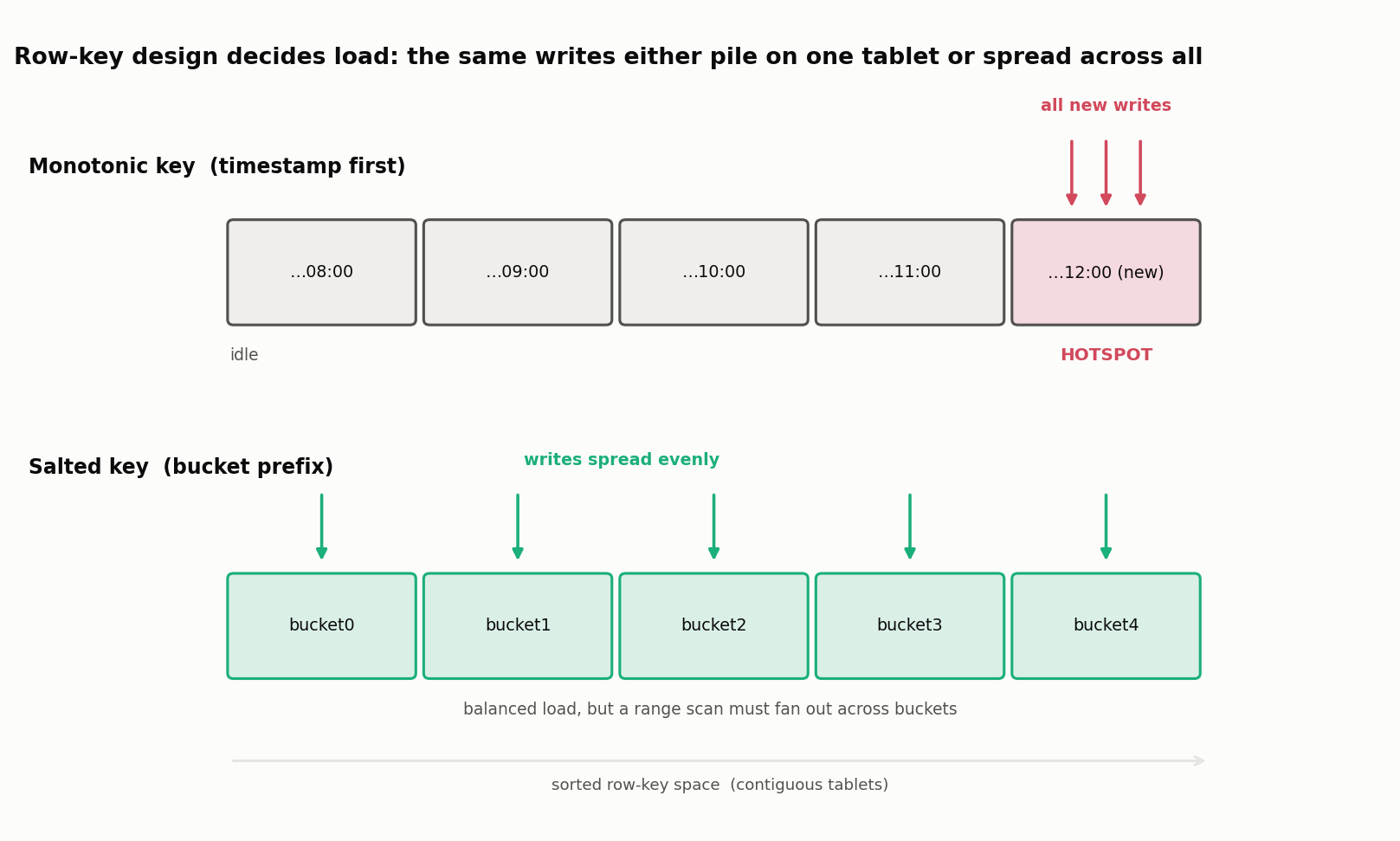
The figure makes the trade-off concrete: the same write load either piles onto one tablet or spreads across all of them, entirely because of a prefix. The right choice depends on the query shape and the traffic distribution, not on a rule.

Fast and Slow Queries

With the model straight, the fast and slow queries follow directly. Fast queries stay aligned to the row key; slow queries abandon it.

Query	Verdict	Why
Point read: get(row_key = 'user_4321')	Fast	Direct lookup of one row in one tablet.
Prefix scan: recent events for device_XYZ	Fast	With an entity-prefixed key, those rows are contiguous, so it reads a small range.
Filter on a non-key column: WHERE country = 'AUS'	Slow	Bigtable has no synchronous secondary index, so this must scan every row on every node.
COUNT(*) or GROUP BY on a non-key column	Slow	A cluster-wide scan and aggregation; the wrong tool for the job.
Writes keyed by a raw timestamp	Slow (hotspot)	Every write targets the newest tablet, so throughput collapses to one node even though it is “by key.”

Note that a prefix scan is not inherently slow. The common claim that “keys starting with A are scattered across the cluster” is only true if the schema deliberately salts them; by default, A-prefixed keys are contiguous. The genuine anti-patterns are querying a non-key attribute and using a monotonic key.

Transactions and Indexes: Design Around the Row

Two limitations shape Bigtable schemas:

• Atomicity is per-row. Bigtable supports atomic single-row reads and writes, but not arbitrary multi-row transactions. The guidance follows directly: keep data that must be read or updated atomically in one row, and avoid spreading it across rows.
• No synchronous secondary indexes. The general-availability pattern for querying by a non-key attribute is to maintain a denormalized lookup table whose row key is that attribute, written alongside the base table. (Bigtable has recently added a pre-GA asynchronous secondary index, an eventually-consistent materialized view, but the denormalized-table pattern remains the default and the one to reach for.)

Consistency Depends on Topology

Bigtable’s consistency is not a fixed property of the product:

• A single-cluster instance is strongly consistent.
• A replicated multi-cluster instance is eventually consistent by default: reads and writes within one cluster are consistent, but across clusters they converge asynchronously.
• Routing changes the guarantee. An app profile with single-cluster routing keeps reads and writes on one cluster (read-after-write behavior); true strong consistency requires routing to a single cluster and using the others only for failover.

This is Part 1’s CAP point in miniature: the same product offers different guarantees depending on topology and routing, so “is Bigtable consistent?” has no answer without those details.

Spanner: Strongly Consistent SQL at Global Scale

Google Cloud Spanner is the database that seems to break the rules: a globally distributed, horizontally scalable, strongly consistent relational database with real ACID transactions and SQL. In one line, it pairs the horizontal scale usually associated with NoSQL with the consistency and query model of a relational database. It is fully managed, and it backs Google-scale systems that need both scale and correctness.

How It Holds Consistency Together

Four mechanisms combine, and it is a mistake (a common one) to credit the clock alone:

1. Key-range splits, synchronously replicated. Spanner shards tables into splits by primary-key range and replicates each split across zones and regions using Paxos quorum consensus. A write commits once a majority of replicas acknowledge it, so a minority failure does not lose data or block progress.
2. TrueTime. Spanner’s TrueTime API exposes bounded clock uncertainty: backed by GPS and atomic clocks, it returns not a timestamp but an interval guaranteed to contain the true time. By waiting out that small uncertainty before committing, Spanner assigns globally meaningful commit timestamps and achieves external consistency (linearizability), the strongest practical consistency guarantee.
3. Two-phase locking provides isolation for read-write transactions (with wound-wait to prevent deadlock).
4. Two-phase commit provides atomicity when a transaction spans multiple splits.

TrueTime is the famous ingredient, but it supplies ordering; the locking, Paxos replication, and two-phase commit supply isolation, durability, and atomicity. The guarantee is the combination.

On the query side, Spanner offers GoogleSQL and a PostgreSQL dialect, with joins, secondary indexes, and change streams. It is important to be precise here: this is two specific dialects, not blanket “ANSI SQL” compatibility.

Spanner and CAP: Highly Available, Not an Exception

The tidy story that Spanner “beats CAP” or “provides all three” is wrong, and Google’s own engineers say so. Spanner is technically a CP system. During a network partition that prevents a quorum, it chooses consistency: the affected operations are rejected or delayed rather than risk serving divergent data.

What confuses people is availability. Spanner targets very high availability (a multi-region configuration aims for five nines, 99.999%), so in practice partitions that would force the trade-off are exceedingly rare, and it feels like a CA system. But CAP-availability is a formal, all-or-nothing property: it requires every request to a non-failing node to succeed even under an arbitrary partition. A 99.999% availability figure, however impressive, is not that. The accurate statement is that Spanner is a highly available, strongly consistent CP database, not an exception to CAP.

Bigtable versus Spanner

They are often shortlisted together and are built for opposite jobs:

Dimension	Bigtable	Spanner
Model	Wide-column NoSQL (sorted key-value)	Distributed relational (SQL)
Schema	Semi-structured, key-designed	Structured, typed, with joins
Transactions	Atomic per row	ACID across rows and tables, global
Consistency	Strong (single cluster); eventual (multi-cluster)	External consistency (linearizable)
Best for	High-throughput key lookups, time-series, feature serving	Global OLTP needing strong consistency: ledgers, inventory, orders
Relative cost	Lower	Premium

The selection rule is short: reach for Bigtable when the workload is key-value lookups and range scans at scale, and for Spanner when the workload needs relational transactions and strong consistency across many rows or regions. Use Spanner’s power only when the problem calls for it; for small datasets, low QPS, or simple lookups, it is expensive overkill, and Bigtable or a single relational database is the better fit.

---

Two systems, two lessons that generalize. Bigtable shows that in a wide-column store the key is the design: placement, scan cost, and hotspots all follow from it. Spanner shows that even the most advanced distributed database does not escape CAP; it engineers the partition case to be rare and chooses consistency when it happens. Both reinforce Part 1’s thesis: understand the access pattern and the failure semantics, and the right store, and the right schema within it, follows.

Resources

• Chang, F. et al. (2006). Bigtable: A Distributed Storage System for Structured Data. OSDI 2006. (Journal version: ACM TOCS 26(2), 2008, doi:10.1145/1365815.1365816.)
• Corbett, J. C. et al. (2012). Spanner: Google’s Globally-Distributed Database. OSDI 2012. (Journal version: ACM TOCS 31(3), 2013, doi:10.1145/2491245.)
• Brewer, E. Inside Cloud Spanner and the CAP Theorem. Google Cloud.
• Bigtable schema design and Spanner: TrueTime and external consistency.