Deep Learning Primer: Diving into the Activation Function Pool

In the architecture of a deep neural network, activation functions are the crucial component that breathes life into the model. Without them, even the deepest network would be nothing more than a single affine transformation in disguise.

In this post, we’ll explore what activation functions are, why they are essential, how their derivatives shape training, and how to choose the right one for our model.

A. What are Activation Functions and Why are They Essential?

An activation function is a mathematical gatekeeper found at the end of every neuron in a neural network. It takes the neuron’s weighted sum input ($z$) and transforms it into an output ($a$), deciding whether the neuron should “fire” (be active) or not.

\[a = f(z) = f(w \cdot x + b)\]

Why are they essential?

The primary purpose of an activation function is to introduce non-linearity into the network. Imagine a neural network without activation functions. Each layer would then be an affine map, $Wx + b$ (linear when the bias $b$ is zero, affine in general), and composing affine maps only ever yields another affine map:

Layer 1: $h_1 = W_1 x + b_1$ (affine)
Layer 2: $h_2 = W_2 h_1 + b_2$ (affine)
Output: $y = W_3 h_2 + b_3$ (affine)

Substituting each equation into the next, the whole network collapses into a single affine map:

\[y = W_3\big(W_2(W_1 x + b_1) + b_2\big) + b_3 = W_{\text{eq}}\, x + b_{\text{eq}}.\]

So a 100-layer “deep” network without activations has exactly the representational power of one affine layer, no more: it can only split the input space with straight boundaries, never curves. Inserting a nonlinear $f$ between layers is what breaks this collapse and lets depth build genuinely richer functions.

This is the setting for the Universal Approximation Theorem, which is worth stating precisely because it is often overstated. It says that a sufficiently wide network with a suitable nonlinear activation can approximate any continuous function on a bounded domain to any desired tolerance. That is an existence result: it guarantees such a network exists, but says nothing about whether training will find it, how much data that would take, or whether it will generalize. Nonlinearity is what makes the approximation possible; it is not a promise that a given finite network learns any target function.

B. Proving Non-Linearity: The ReLU Example

A function $f(x)$ is linear if and only if it satisfies two properties:

Additivity: $f(x + y) = f(x) + f(y)$
Homogeneity: $f(\alpha x) = \alpha f(x)$

Let’s test this on ReLU (Rectified Linear Unit), which is defined as $f(x) = \max(0, x)$.

Test 1: Additivity

Let $x = 5$ and $y = -5$.
$f(x + y) = f(5 + -5) = f(0) = \mathbf{0}$
$f(x) + f(y) = f(5) + f(-5) = 5 + 0 = \mathbf{5}$
Result: $0 \neq 5$. Additivity fails.

Test 2: Homogeneity

Let $x = 5$ and $\alpha = -1$
$f(\alpha x) = f(-5) = \mathbf{0}$
$\alpha f(x) = -1 \cdot f(5) = -1 \cdot 5 = \mathbf{-5}$
Result: $0 \neq -5$. Homogeneity fails.

Because it fails these tests, ReLU is mathematically non-linear. By stacking layers of ReLU neurons, a network can bend and fold the feature space to solve complex problems that a linear model never could.

C. Major Activation Functions: Formulations & Analysis

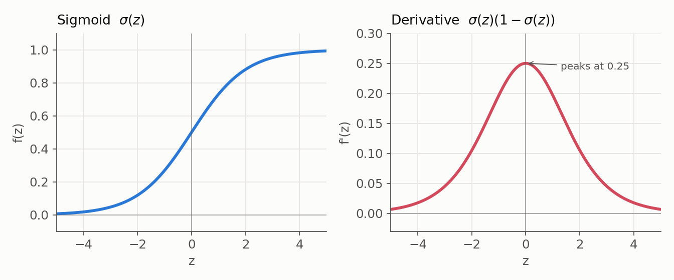
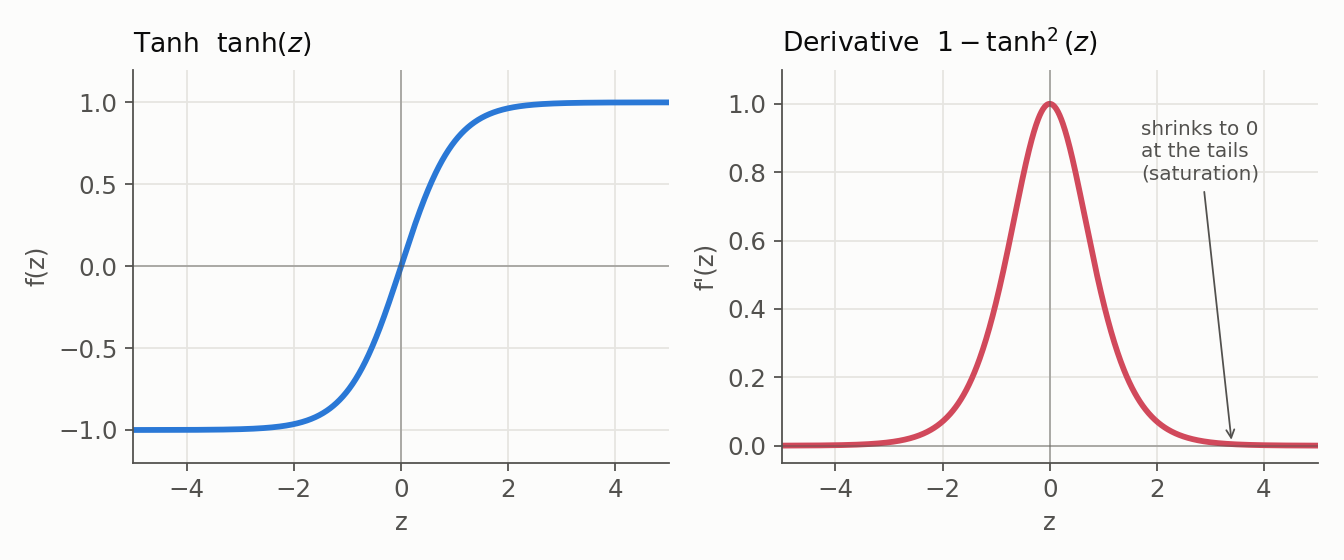
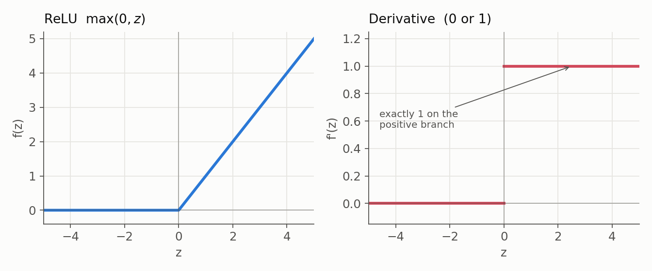
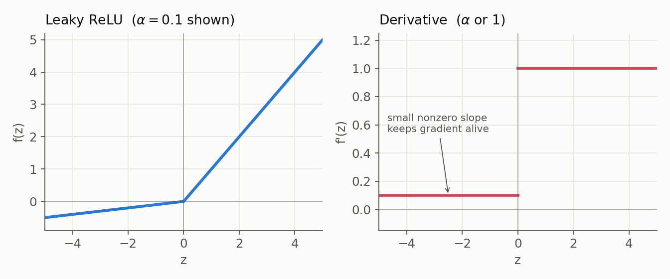
For training, a function’s derivative matters as much as its formula: backpropagation multiplies these derivatives layer by layer, so wherever a derivative is near zero, the gradient shrinks and learning stalls. For each function below we plot the activation next to its first derivative; watch the derivative panel, because that is where saturation (a derivative decaying to zero) becomes visible.

1. Sigmoid (Logistic)

• Formula: $\sigma(z) = \frac{1}{1 + e^{-z}}$
• Derivative: $\sigma’(z) = \sigma(z)\,(1 - \sigma(z))$, which peaks at only $0.25$ (at $z = 0$) and decays to $0$ as $\lvert z\rvert$ grows.
• Range: $(0, 1)$; not zero-centered, since outputs are always positive.
• Use Case: A probability at the output layer of binary classification, or a gate inside an LSTM.
• Issues:
  • Saturation: for large $\lvert z\rvert$ (say $z = 10$ or $z = -10$) the derivative is near zero, so gradients through a saturated sigmoid shrink sharply. With a peak derivative of $0.25$, stacking sigmoids multiplies these small factors, a classic route to vanishing gradients.
  • Not zero-centered: always-positive outputs make the next layer’s weight gradients share a sign, which can cause zig-zagging updates.

2. Tanh (Hyperbolic Tangent)

• Formula: $\tanh(z) = \frac{e^z - e^{-z}}{e^z + e^{-z}}$
• Derivative: $1 - \tanh^2(z)$, peaking at $1$ (at $z = 0$) and again decaying to $0$ at the tails.
• Range: $(-1, 1)$; zero-centered, which is its main advantage over Sigmoid and tends to make optimization easier.
• Issue: Still saturates for large $\lvert z\rvert$, so deep stacks of Tanh can still vanish gradients, just less aggressively than Sigmoid.

3. ReLU (Rectified Linear Unit)

• Formula: $f(z) = \max(0, z)$
• Derivative: $1$ for $z > 0$ and $0$ for $z < 0$; undefined at exactly $z = 0$, where software picks a subgradient by convention (commonly $0$).
• Range: $[0, \infty)$; not zero-centered.
• Benefit: Cheap to compute (a single max), and its positive-branch derivative of $1$ does not shrink the signal the way a saturating unit does, so ReLU networks typically train faster than Sigmoid or Tanh ones.
• Issue: “Dying ReLU”. A unit whose pre-activation is negative for all relevant inputs receives zero gradient through the ReLU and stops updating from that path. This is a risk, not a life sentence: a change in upstream weights, biases, or normalization statistics can move the pre-activation back into the positive region and revive the unit. A too-large learning rate or a strongly negative bias makes it more likely.

4. Leaky ReLU

• Formula: $f(z) = \max(\alpha z, z)$ with $\alpha$ small and fixed (e.g. $0.01$).
• Derivative: $1$ for $z > 0$ and $\alpha$ for $z < 0$, so a small gradient always flows.
• Benefit: Softens the dying-ReLU risk by keeping a nonzero slope on the negative branch.

5. ELU (Exponential Linear Unit)

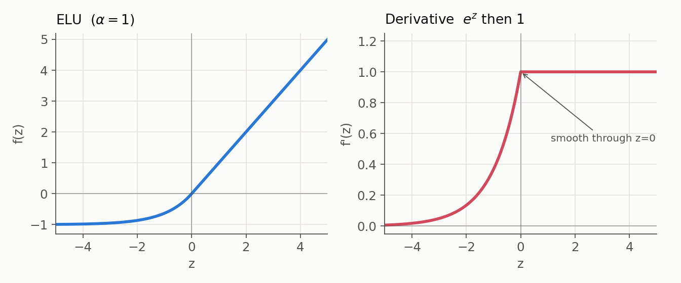
• Formula: $f(z) = z$ for $z > 0$, else $\alpha(e^z - 1)$.
• Derivative: $1$ for $z > 0$, and $\alpha e^z$ for $z < 0$; smooth through $z = 0$ when $\alpha = 1$.
• Range: $(-\alpha, \infty)$.
• Benefit: The smooth negative branch pushes mean activations toward zero, which can speed learning.
• Issue: The $e^z$ term makes it costlier than ReLU.

6. GELU (Gaussian Error Linear Unit)

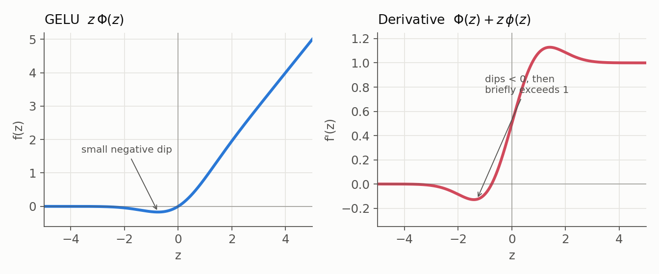
• Formula: $f(z) = z\,\Phi(z)$, where $\Phi$ is the standard-normal CDF (often computed via a tanh approximation).
• Derivative: $\Phi(z) + z\,\phi(z)$, smooth everywhere; it dips slightly below zero for small negative $z$ and can briefly exceed $1$.
• Range: approximately $(-0.17, \infty)$; non-monotonic, with a small negative dip near $z \approx -1$.
• Context: The default activation in the feed-forward blocks of most Transformers (BERT and the GPT family). It behaves like a smoothed ReLU that lets a little negative signal through, weighting each input by roughly the probability that a standard normal falls below it.

7. SiLU / Swish

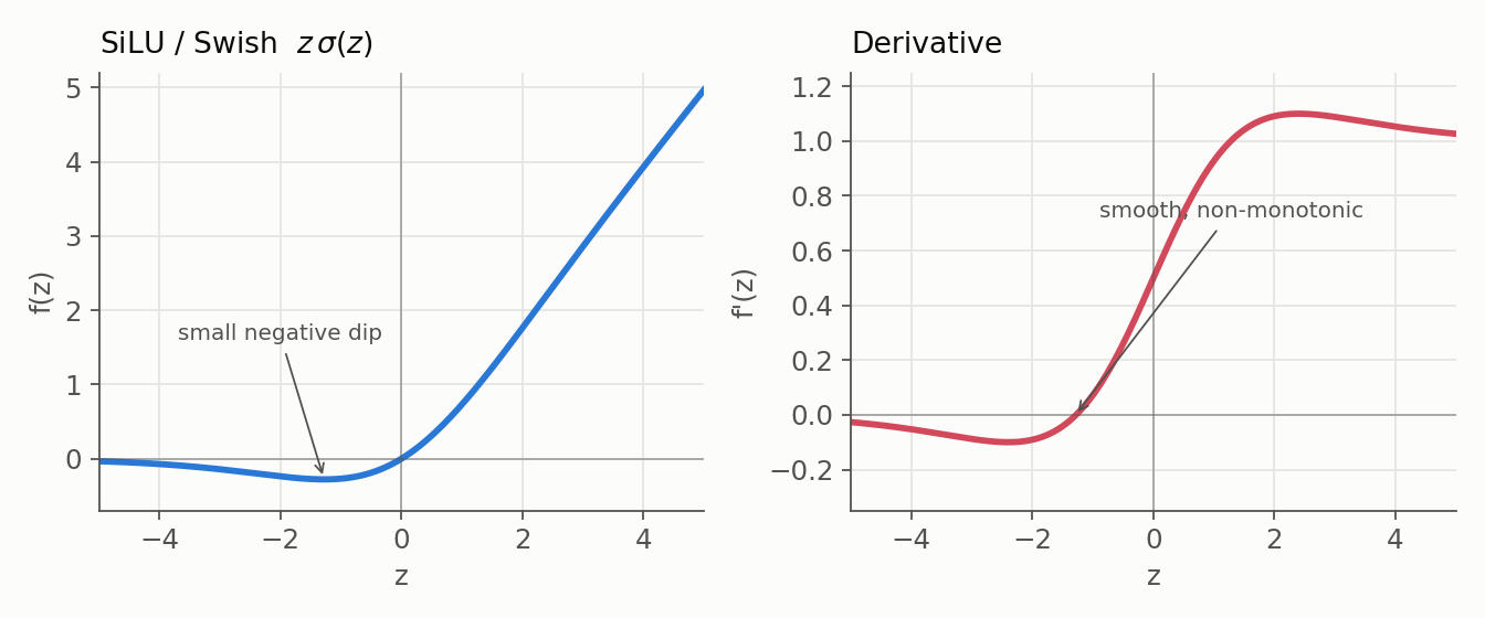
• Formula: $f(z) = z\,\sigma(z)$ (the Sigmoid-weighted linear unit; “Swish” is the same function).
• Derivative: $\sigma(z) + z\,\sigma(z)(1 - \sigma(z))$, smooth and, like GELU, non-monotonic.
• Range: approximately $(-0.28, \infty)$.
• Context: Close in shape to GELU, and common in vision models (EfficientNet) and several LLMs. Smoothness plus a small negative region is the shared theme of the modern units.

8. PReLU (Parametric ReLU)

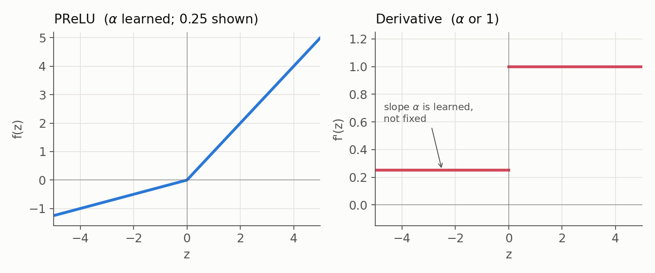
• Formula: $f(z) = \max(\alpha z, z)$, the same shape as Leaky ReLU but with $\alpha$ learned (often per channel) rather than fixed.
• Benefit: Lets the network choose how much negative signal to keep, at the cost of a few extra parameters.

Gated blocks are not scalar activations. Variants like GLU and SwiGLU are not point-wise functions of a single $z$. A gated block splits a layer into two projections and multiplies one by an activation of the other, for example $\text{SwiGLU}(x) = \text{SiLU}(xW_1) \odot (xW_2)$. They show up in modern Transformer feed-forward layers and often replace a plain activation there, but they are a block built from projections and an element-wise gate, not a drop-in scalar nonlinearity.

9. Softmax (a vector function, not a scalar activation)

• Formula: for a vector of logits $z = (z_1, z_2, \dots, z_K)$,

\[\text{softmax}(z)_i = \frac{e^{z_i}}{\sum_{j=1}^{K} e^{z_j}}.\]

• Range: each component in $(0, 1)$, and the components sum to $1$.
• Use Case: Turning $K$ logits into a distribution over mutually exclusive classes for single-label multiclass problems. The very same operation also appears inside models, most notably in attention, where it normalizes scores into weights, so softmax is not only an output-layer device.
• Caveat: A softmax output is the model’s probability, not a guarantee of calibrated confidence; a model can be confidently wrong, and calibration is a separate property to measure. For multilabel problems, where several labels can be true at once, a per-label Sigmoid is the right choice rather than Softmax.

D. The Power of Asymmetry (ReLU & ELU)

ReLU and ELU are asymmetric functions (they behave differently for positive vs. negative inputs). This asymmetry is often useful, though the usual claims about it deserve care.

Sparsity (ReLU): Because ReLU outputs exactly $0$ for negative pre-activations, some fraction of hidden units are inactive on any given input, producing a sparse activation pattern. That fraction is not a fixed “50% or more”: it depends on the learned weights, biases, normalization, and the data, and shifts as the network trains. And exact zeros in a dense layer do not by themselves save computation, because a standard dense kernel still multiplies through them. Turning activation sparsity into a real speedup requires compatible sparse storage and kernels, which most training setups do not use.

Specialization: Networks can learn to route different inputs through different active subnetworks, one path lighting up for one kind of feature while others stay at zero. This is a plausible learned representation that gating-style activations encourage, not a direct mathematical consequence of asymmetry; whether it happens depends on what the network actually learns.

E. Tackling Exploding and Vanishing Gradients

The activation function is one influence on gradient flow, not the only one. The gradient that reaches an early layer is a product of activation derivatives and weight matrices and any normalization Jacobians, so activations, initialization, and normalization work together, and no single one of them fixes gradient problems on its own.

1. The Vanishing Gradient Problem

Cause: In deep networks with Sigmoid/Tanh, the per-layer activation derivatives are all below $1$ (at most $0.25$ for Sigmoid), and multiplying many of them through the chain rule drives the gradient toward zero. The early layers then barely learn.

How ReLU helps, and its limits: On its active positive branch ReLU has derivative $1$, so it does not shrink the signal the way a saturating unit does, which is a large part of why deep ReLU networks train more readily. But this is not a proof that gradients cannot vanish or explode: the same backpropagated gradient still carries the products of the weight matrices and normalization terms, and units sitting on their negative branch contribute exactly zero. ReLU removes one source of shrinkage; it does not remove the others.

2. The Exploding Gradient Problem

Cause: Repeated multiplication by factors greater than one (large weights, especially) makes gradients grow without bound, so weights update wildly and the loss can go to NaN.

Solutions (a stack, not a single fix):

• Gradient Clipping: cap the gradient norm (e.g. at $1.0$) during training, a direct guard against explosion.
• Weight Initialization: use He initialization for ReLU-family units and Xavier/Glorot for Sigmoid/Tanh, so the variance of activations stays roughly stable across layers at the start of training.
• Normalization: BatchNorm (or LayerNorm) standardizes a layer’s summed inputs to zero mean and unit variance, then applies a learned shift and scale. That keeps pre-activations in a stable range and reduces sensitivity to initialization. Note what it does not do: it centers values around zero, rather than pushing them into any activation’s positive range.

A Note on Scaling, Initialization, and Normalization

These are three separate choices that are easy to conflate:

• Feature scaling (standardizing the inputs) improves the conditioning of the optimization for essentially any network; it is a property of good preprocessing, not a yes/no flag attached to a particular activation.
• Weight initialization sets the starting variance of signals so they neither vanish nor explode on the first forward and backward pass.
• Hidden-state normalization (BatchNorm/LayerNorm) keeps intermediate activations well-behaved during training.

The next posts in this primer take up initialization and normalization in their own right.

F. Output Activations and Their Losses

A useful discipline is to separate hidden activations (chosen for gradient flow and expressivity) from output activations (chosen to match the task and its loss). The output layer’s job is to produce exactly the representation the loss expects.

Task	Typical output	Typical loss
Regression	Identity (a raw value), or a constrained transform such as softplus for positive targets	MSE, MAE, or a likelihood loss
Binary label	One logit; apply Sigmoid only when an explicit probability is needed	Binary cross-entropy (from logits)
Single-label multiclass	$K$ logits, Softmax conceptually	Cross-entropy (from logits)
Multilabel	$K$ independent logits, one Sigmoid each	Binary cross-entropy per label (from logits)

One practical point ties the table together: numerically stable libraries usually fuse the final activation into the loss rather than asking us to apply Sigmoid or Softmax first. PyTorch’s BCEWithLogitsLoss and CrossEntropyLoss take logits directly and apply the exponential internally with the log-sum-exp trick, avoiding the overflow and precision loss of computing a probability and then its logarithm separately. The rule of thumb: keep the final layer as raw logits, and let the loss function apply the exponential.