Deep Learning Primer: Understanding Word Embeddings: From SVD to Word2Vec
How do we represent the meaning of a word to a computer? This is the fundamental question of Natural Language Processing. Simply treating words as unique IDs fails to capture the relationships between them (e.g., that “chair” and “seat” are similar).
This post explores the journey of word representations, starting from classical statistical methods and evolving into the neural-based Word2Vec models (CBOW and Skip-Gram).
The Co-occurrence Matrix
The intuition behind word representation is distributional semantics: a word is defined by the company it keeps. We start by building a Co-occurrence Matrix of dimension $V \times V$ (where $V$ is the vocabulary size).
For every candidate word, we define a “context window” of size $k$. We count how many times context words appear within that window around the candidate word across the entire corpus.
Fixable Problems with Raw Counts
Raw counts have issues. “The”, “a”, and “is” appear everywhere but carry little semantic weight. We suggest three solutions:
- Stop words: Simply remove very frequent words.
- Thresholding: Cap the counts using $x_{ij} = \min(count(w_i, c_j), t)$ where $t$ is the threahold count, e.g. 100.
PMI (Pointwise Mutual Information): Instead of raw counts, use PMI to measure how likely words occur together compared to chance.
\[PMI(w, c) = \log \frac{P(w, c)}{P(w)P(c)} = \log \frac{count(w, c) * N}{count(w) * count(c)}\]$N$ is the total number of words.
Since $\log(0)$ is problematic, we often use PPMI (Positive PMI), where negative values are floored at 0.
Part 1: The Classical Approach (Count-Based)
Dimensionality Reduction via SVD
The resulting matrix $X (= X_{PPMI})$ is sparse and high-dimensional ($V \times V$). We need a dense, lower-dimensional representation. We apply Singular Value Decomposition (SVD): \(X = U \Sigma V^T\)
According to the SVD theorem, if we truncate the matrices to keep only the top $k$ singular values (rank-$k$ approximation), we preserve the most important information while compressing the data.
An Analogy for Compression:
Imagine representing colors using 8 bits where leftmost 4 bits store intensity and rightmost 4 bits store the actual color. “Very light green” and “light green” have different codes for leftmost 4 bits, but same codes for rightmost 4 bits. If asked to compress this to 4 bits, we retain only the rightmost 4 bits, and lose information on the intensity because getting the color right in this reduced dimension is more important than getting the intensity.
If we apply SVD on $X_{PPMI}$ and get \(\hat{X} = (U_{m,k}\Sigma_{k,k}V^{T}_{k,n})\) after keeping only the top-$k (k \ll n)$ singular values, the sparse co-occurance matrix would become dense. Some co-occurances which previously were not captured, would now start to get captured.
- Recall that each row in the original matrix $X$ served as the representation of a word.
- Then $XX^T$ would result in a matrix whose $(i,j)^{th}$ entry would be the dot-product between the representation of word $i$ and $j$.
Once we perform SVD, what’s a good choice for the word representation?
- Obviously taking the $i^{th}$ row of the reconstructed matrix $\hat{X}$ doesn’t make sense because it’s still high dimensional.
- But we saw that the reconstructed matrix $\hat{X} = U \Sigma V^{T}$ discovers latent semantics and its word representations are more meaningful. In general \((XX^T)_{ij} \le (\hat{X}\hat{X}^T)_{ij}\).
Wishlist
We’d want representation of each word with much lesser dimension (compared to $V$), but still maintatin similarity scores like $(\hat{X}\hat{X}^T)_{ij}$.
Notice that the dot product between the rows of the matrix $W_{word} = U\Sigma$ is the same as the dot product between the rows of $\hat{X}$.
\[\hat{X}\hat{X}^T = (U \Sigma V^{T})(U \Sigma V^{T})^{T}\] \[= (U \Sigma V^{T}) \cdot (V \Sigma^{T} U^{T})\] \[= (U \Sigma) \cdot (\Sigma^{T} U^{T})\] \[= (U \Sigma) \cdot (U \Sigma)^{T}\] \[= W_{word} \cdot W_{word}^{T}\]\(\hat{X} \in \mathbb{R}^{m*n}\) but \(W_{word} \in \mathbb{R}^{m*k}\), and we’ve $k \ll n$. This serves our purpose.
Conventionally, \(W_{word} = U\Sigma (\in \mathbb{R}^{m*k})\) is taken as the word-represenation and \(W_{context} = V (\in \mathbb{R}^{n*k})\) is taken as representation of the context words.
Part 2: The Neural Approach (Word2Vec): Continuous Bag of Words (CBOW)
While SVD is powerful, it is computationally expensive to update as the vocabulary grows. This motivates “prediction-based” models like CBOW/SkipGram.
Let’s write out the complete CBOW training procedure step-by-step for a single-sentence corpus using a context window of 2.
1. Corpus and training examples
Take the sentence (example):
1
A quick brown fox jumps over the lazy dog
Vocabulary (V) = unique words in the corpus (here 9 words). Window size (w = 2) means we use up to 2 words on each side as context.
For each token at position (t) (except edges), create a training sample:
- Context ($C_t = {x_{t-2}, x_{t-1}, x_{t+1}, x_{t+2}}$) (some positions may have fewer than 4 if near edges)
- Target ($y_t = x_t$)
Examples of training pairs (position → (context, target)):
- t=3 (“brown”): context = [“A”,”quick”,”fox”,”jumps”], target = “brown”
- t=4 (“fox”): context = [“quick”,”brown”,”jumps”,”over”], target = “fox”
- etc.
We turn each word into a one-hot column vector:
\[u \in \mathbb{R}^{V \times 1}\]where exactly one entry is 1.
2. CBOW DNN architecture (mathematical)
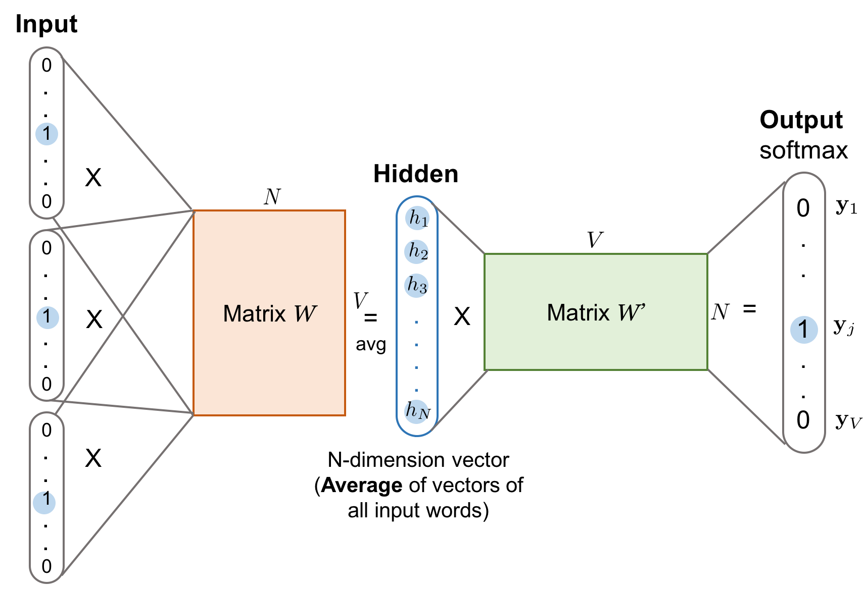
Image credit: https://deeplearning.ir/wp-content/uploads/2019/05/word2vec-cbow.png
Parameters to learn:
- Input embedding matrix $W \in \mathbb{R}^{n \times V}$. Each column = embedding of a word. Embedding dimension = (n).
- Output weight matrix $W’ \in \mathbb{R}^{V \times n}$ (or classifier matrix). This maps an (n)-dim vector back to vocab space..
Notation:
- Vocabulary size ($V$)
- Embedding dim ($n$)
- Number of context words $(m = \lvert C_t \rvert)$ (here up to 4)
3. Forward Pass for One Training Example
Let context have (m) words (usually 4).
Step 1: Get embeddings for each context word
For each context word with one-hot $(u_i)$:
\[e_i = W_{in} u_i \quad (n \times 1)\]This selects the corresponding $i^{th}$ column from $W$.
Step 2: Average embeddings
\[h = \frac{1}{m} \sum_{i=1}^m e_i \quad (n \times 1)\]This is the hidden CBOW representation.
Step 3: Compute logits (scores for all words)
\[z = W' h \quad (V \times 1)\]Step 4: Softmax prediction
\[\hat{y}_j = \frac{e^{z_j}}{\sum_{k=1}^{V} e^{z_k}}\]4. Loss/Gradients/Backprop
The “math” of the gradient descent (Chain Rule) is identical to standard deep learning, but the mechanics of how the updates are applied in CBOW are distinct in two critical ways.
Here are the key differences between a standard Feed-Forward Network (MLP) and CBOW:
1. Sparse vs. Dense Updates (The “Lookup” Difference)
In a standard Neural Network (e.g., predicting housing prices from 10 features), every weight in the first layer contributes to the output, so every weight gets an update during every iteration.
In CBOW, the input is a Lookup Table.
- Standard NN: $\nabla W$ is a dense matrix. All $N \times M$ weights change slightly.
- CBOW: $\nabla W$ is incredibly sparse.
- If your vocabulary $V$ is 100,000 and your context size is 4, you only touch 4 rows of the input matrix $W$.
- The other 99,996 rows have a gradient of exactly 0.
- Implication: You don’t perform matrix multiplication for the backward pass on $W$; you perform “row indexing” and “vector addition.”
- During backpropagation in CBOW, the gradient flows only through the context embeddings (the columns of $W$ selected by the context words). Since the target word’s embedding is not used in predicting itself, its column in $W$ receives no gradient update. Only the relevant context columns get updated.
2. Identical Gradients (The “Averaging” Difference)
In a standard MLP, the first layer usually multiplies input features by different weights ($x_1 w_1 + x_2 w_2$). The network learns that Feature 1 is more important than Feature 2, so $w_1$ and $w_2$ get different gradients.
In CBOW, we average the word vectors before the hidden layer: \(h = \frac{v_1 + v_2 + \dots + v_c}{C}\)
Because of this summing/averaging operation, the “back-propagated error” ($EH$) that arrives at the hidden layer is distributed equally to all context words.
- Result: $\nabla v_{quick} = \nabla v_{brown} = \nabla v_{jumps} = \nabla v_{over}$
- Implication: In a single training step, the model cannot distinguish which word contributed more to the prediction. It assumes all context words are equally responsible for the target. It is only over many epochs with different contexts that the vectors differentiate.
3. Positional Agnosticism
In a standard sequence model (like an RNN or a Transformer) or even a standard MLP, the position matters.
- Input 1 is “Subject”, Input 2 is “Verb”.
- Weights are learned specific to those positions.
In CBOW, because of the summation/averaging gradient:
- Context
["The", "cat"]produces the exact same gradient update as["cat", "The"]. - The gradient descent process in CBOW is invariant to the order of context words. It creates a “Bag of Words” representation where spatial information is explicitly discarded during the update.
Summary Table
| Feature | Standard MLP Backprop | CBOW Backprop |
|---|---|---|
| Input Weights | Dense Matrix Multiplication | Row Lookup / Indexing |
| Update Scope | All weights updated every step | Only $C$ rows updated (Sparse) |
| Gradient Value | Unique for every input feature | Identical for all active context words |
| Word Order | Usually preserved (via different weights) | Lost (Order doesn’t affect gradient) |
In CBOW, synonyms appear in similar contexts; since the model uses those contexts to update word vectors, synonymous words receive nearly identical gradient updates, causing their embeddings to move closer together in the vector space.
Technical Note on Efficiency: Because of “Difference #1” (Sparsity), standard deep learning frameworks (like PyTorch/TensorFlow) often use a specialized layer (e.g., nn.Embedding) instead of a standard nn.Linear layer. nn.Embedding is optimized to handle these sparse gradient updates without calculating the zeros for the rest of the vocabulary.
Part 3: The Neural Approach (Word2Vec): The Skip-Gram Model
1. What is Skip-Gram?
Skip-Gram is one of the core Word2Vec architectures. Its goal is the opposite of CBOW:
Skip-Gram predicts the surrounding context words given the center (target) word.
If the sentence is:
1
A quick brown fox jumps over the lazy dog
and the center word is “brown” with window size 2, then Skip-Gram tries to predict:
1
{ "quick", "fox" }
CBOW: context → target Skip-Gram: target → context
2. Skip-Gram Model Architecture
Embedding matrices (column-wise convention)
Input embeddings:
\[W \in \mathbb{R}^{n \times V}\](columns = embeddings)
Output embeddings:
\[W' \in \mathbb{R}^{V \times n}\]
Training pairs in Skip-Gram
For a target word (x_t) and window (w):
\[(x_t, x_{t-2}), (x_t, x_{t-1}), (x_t, x_{t+1}), (x_t, x_{t+2})\]So one target produces multiple training examples.
3. Forward pass
- Represent center word as one-hot vector $(u_c)$
Embed:
\[h = W[:,c] \in \mathbb{R}^{n}\]For each context word ($k$):
\[z_k = W'[k,:] \cdot h\]Use softmax:
\[P(\text{context}=k \mid \text{center}=c) = \frac{e^{z_k}}{\sum_{j=1}^{V} e^{z_j}}\]
Key Differences Between Skip-Gram and CBOW
| Aspect | CBOW | Skip-Gram |
|---|---|---|
| Direction | context → target | target → context |
| Training pairs | 1 per target | multiple per target |
| Input | average of context embeddings | embedding of center word |
| Updates to embeddings | context embeddings only | center embedding + sampled outputs |
| Works well with | large corpus, frequent words | small datasets, infrequent words |
| Training speed | faster (only 1 softmax per target) | slower (multiple predictions per target) |
| Embedding stability | smoother, averaged representations | richer, more detailed representations |
| Rare words | performs worse | performs better |
| Use case | fast training, general semantics | high-quality embeddings, small corpora |
When to Choose Which?
Use CBOW when:
- You have a very large dataset
- You want fast training
- You care about stable/average meanings (e.g., “bank” often becomes the average of contexts)
Use Skip-Gram when:
- You want high-quality embeddings
- You want to capture more subtle relations
- You have a smaller dataset
- You want better performance for rare words
Skip-Gram tends to produce richer, more nuanced embeddings.
The Computational Bottleneck
The “Computational Bottleneck” comes from the denominator of the Softmax function. To update the weights for one word (like “fox”), we currently have to calculate the dot product for every single word in the dictionary (100,000+) to normalize the probability. This makes training on large datasets impossible.
Negative Sampling (NEG) solves this by changing the fundamental question the model asks.
1. The Core Idea: Changing the Problem
Instead of a massive Multi-Class Classification problem (“Out of 100,000 words, which one is it?”), Negative Sampling turns it into a set of small Binary Classification problems (“Is this specific word pair real or fake?”).
We no longer want to ensure the probabilities sum to 1. We just want the model to output:
- High probability (1) for the True pair (Context + Target).
- Low probability (0) for a few random Noise pairs (Context + Random Word).
2. The New Training Data
For the sentence “A quick brown fox…” with target “fox”:
The Positive Sample (Label = 1):
- Input:
["A", "quick", "brown", "jumps"]$\rightarrow$ Target: “fox” - Objective: Maximize sigmoid($h \cdot u_{fox}$)
The Negative Samples (Label = 0): We randomly pick $K$ words from the vocabulary (usually $K=5$ to $20$) that are not the target. Let’s say we pick “apple”, “car”, and “tennis”.
- Input:
["A", "quick", "brown", "jumps"]$\rightarrow$ Target: “apple” - Input:
["A", "quick", "brown", "jumps"]$\rightarrow$ Target: “car” - Input:
["A", "quick", "brown", "jumps"]$\rightarrow$ Target: “tennis” - Objective: Minimize sigmoid($h \cdot u_{neg}$)
3. The New Loss Function
We replace the Softmax Cross-Entropy with the Negative Sampling Loss:
\[J(\theta) = - \log \sigma(h \cdot u_{target}) - \sum_{k=1}^{K} \log \sigma(- h \cdot u_{neg_k})\]- First term: We want the probability of the real word to be close to 1.
- Second term: We want the probability of the negative words to be close to 0 (which is mathematically equivalent to maximizing $\sigma(-x)$).
4. How the Gradient Descent Changes
This is where the magic happens.
In Standard Softmax: We had to update the output vector $u_w$ for all 100,000 words because every word appeared in the denominator.
In Negative Sampling: We only update the weights for:
- The 1 positive word (“fox”).
- The $K$ negative words (“apple”, “car”, “tennis”).
The Update Sparsity: If vocabulary $V = 100,000$ and $K=5$:
- Softmax: 100,000 updates per step.
- Negative Sampling: 6 updates per step.
This creates a massive speedup (orders of magnitude), making it possible to train on Google-scale datasets.
5. Smart Sampling (The “Unigram” Trick)
How do we pick the negative words? We don’t pick them purely randomly.
If we pick random words uniformly, we might rarely pick very common words like “the” or “and” as negatives, even though they provide little signal. If we pick strictly by frequency, we might only pick “the” and “and”, and never learn to distinguish “fox” from “wolf”.
Word2Vec uses a “Unigram Distribution raised to the 3/4 power”: \(P(w) = \frac{count(w)^{0.75}}{\sum_{w' \in V} count(w')^{0.75}}\)
Why 0.75? It slightly “flattens” the distribution.
- It dampens the probability of extremely frequent words (like “the”).
- It increases the probability of picking rarer words (like “zebra”) as negatives.
- This ensures the model learns to distinguish the target from a diverse range of incorrect words.
Summary
Negative Sampling is an approximation. We are strictly no longer maximizing the likelihood of the corpus. However, it turns out that for learning high-quality word embeddings, distinguishing the “real” word from 5 “noise” words is sufficient to learn the semantic relationships we care about.