Deep Learning Primer: Exploring Optimization/Stabilization Techniques in DNN

Optimization and stabilization techniques for DNNs focus on training stability (making sure the model actually learns without diverging) and optimization efficiency (reaching the best solution faster).

Top 5 Optimzation & Stabilization Techniques

1. Weight Initialization Strategies (He & Xavier)

Before the network sees a single data point, the starting values of its weights determine whether training will be smooth or impossible. Poor initialization leads to vanishing or exploding gradients almost immediately.

• The Problem: If weights are initialized too small, signals shrink as they pass through layers (vanishing). If too large, signals grow uncontrollably (exploding).
• The Solution: Use mathematically derived variance scaling to keep signal magnitudes constant across layers.
  • Xavier (Glorot) Initialization: Best for Sigmoid or Tanh activation functions. It sets weights based on the number of inputs and outputs of the layer.
  • He (Kaiming) Initialization: Best for ReLU (and its variants) activation functions. It accounts for the fact that ReLU zeroes out half the inputs, requiring slightly larger initial weights to maintain signal variance.

2. Normalization Layers (Batch Norm & Layer Norm)

Deep networks suffer from Internal Covariate Shift, where the distribution of inputs to a layer keeps changing as the previous layers update. This forces the network to constantly “re-learn” how to handle inputs, slowing down training.

• Batch Normalization (BN): Normalizes inputs across the batch dimension.
  • Best for: CNNs and standard feed-forward networks.
  • Benefit: Allows for much higher learning rates and acts as a mild regularizer.
• Layer Normalization (LN): Normalizes inputs across the feature dimension for a single sample.
  • Best for: RNNs and Transformers (where batch dependency is problematic).
  • Benefit: Stabilizes training in sequence models where batch statistics can be noisy or undefined.

3. Residual Connections (Skip Connections)

As networks get deeper (e.g., 50+ layers), accuracy often saturates and then degrades, not because of overfitting, but because the optimization becomes too difficult (the degradation problem).

• The Technique: Instead of learning a mapping $H(x)$ directly, the layer learns a residual mapping $F(x) = H(x) - x$. The output becomes $x + F(x)$.
• Why it works: It creates “gradient superhighways.” During backpropagation, the gradient can flow essentially unaltered through the skip connection to earlier layers. This drastically reduces the vanishing gradient problem and allows extremely deep networks (like ResNet-152 or GPT-4) to be trainable.

4. Adaptive Optimizers (AdamW)

Standard Stochastic Gradient Descent (SGD) uses a fixed learning rate for all parameters, which can be problematic when some parameters need to change enormous amounts while others need tiny tweaks.

• The Technique: Adaptive optimizers adjust the learning rate for each individual parameter based on the history of gradients.
• Top Choice: AdamW (Adam with Weight Decay).
  • Why: It combines the speed of Adam (using momentum and squared gradients to scale learning rates) with correct Weight Decay regularization. This stabilizes training on complex landscapes where standard SGD might get stuck in saddle points or oscillate wildly.

5. Gradient Clipping

Even with good initialization, gradients can occasionally spike (especially in RNNs or very deep networks), causing massive weight updates that “break” the model (the loss suddenly becomes NaN or infinity).

• The Technique: Before updating weights, check the norm (magnitude) of the gradient vector. If it exceeds a threshold (e.g., 1.0), scale the whole vector down so its norm equals that threshold.
• Why it works: It prevents the “exploding gradient” problem physically. It acts as a safety rail, ensuring that no single bad batch of data can destabilize the entire training history.

Comparison Table for Quick Reference

Technique	Primary Role	Best Use Case
He/Xavier Init	Foundation	Essential for all deep nets at the start.
Batch/Layer Norm	Stabilizer	BN for Images/CNNs; LN for Text/RNNs.
Residual connections	Enabler	Essential for very deep networks (>20 layers).
AdamW	Accelerator	The default optimizer for most modern tasks.
Gradient Clipping	Safety Net	RNNs, LSTMs, and unstable training loops.

• We’ve discussed AdamW in our Optimizers article, so we’ll be skipping that.
• We’ll cover Batch-Normalization in the next article as it’s more of a Regularizer.
• Residual Connections will probably need a separate article as there’s quite a lot to unpack there. Also, gradient clipping is a straight-forward mechanism, so we’ll skip that too.

This leaves us with two remaining optimization techniques: He/Xavier Initialization and Layer Normalization. Let’s dig deep into these two.

A Deep Dive into He/Xavier Initialization

Here is a detailed breakdown of He and Xavier initialization, structured for your blog post.

1. Motivation: The “Goldilocks” Zone of Signal

In Deep Neural Networks, the way we initialize weights acts as the foundation for the entire training process. If we initialize weights randomly without a strategy (e.g., using a standard Gaussian distribution $N(0, 1)$), we almost immediately run into one of two catastrophes:

1. Vanishing Gradients: If weights are too small, the signal shrinks as it passes through each layer. By the time it reaches the end, the activation is effectively zero. During backpropagation, the gradients (which are proportional to these activations) also become zero, and the network stops learning.
2. Exploding Gradients: If weights are too large, the signal grows exponentially with every layer. This causes activations to saturate (hitting the flat parts of Sigmoid/Tanh) or go to infinity (ReLU), leading to NaN loss values.

The Goal: We want the variance of the activations to remain constant across every layer. The signal shouldn’t amplify or diminish; it should stay in the “Goldilocks” zone to ensure stable gradients flow during both the forward and backward passes.

2. Mathematical Formulation and Derivations

Let’s derive the condition required to keep the variance stable. Consider a single linear neuron (or a layer in matrix form):

\[y = w_1x_1 + w_2x_2 + \dots + w_n x_n + b\]

For initialization, we assume:

• Biases $b = 0$.
• Weights $w$ and Inputs $x$ are independent random variables.
• Weights and Inputs have a mean of zero ($E[w]=0, E[x]=0$).

We want to find the variance of the output $y$:

\[Var(y) = Var\left(\sum_{i=1}^{n_{in}} w_i x_i\right)\]

Since $w_i$ and $x_i$ are independent, the variance of the sum is the sum of the variances:

\[Var(y) = \sum_{i=1}^{n_{in}} Var(w_i x_i)\]

Using the property $Var(AB) = E[A^2]E[B^2] - (E[A]E[B])^2$, and knowing means are zero:

\[Var(y) = \sum_{i=1}^{n_{in}} Var(w_i) Var(x_i)\]

Assuming all weights and inputs share the same variance properties:

\[Var(y) = n_{in} \cdot Var(w) \cdot Var(x)\]

The Stability Constraint: To prevent the signal from exploding or vanishing, we want the variance of the output to equal the variance of the input: $Var(y) = Var(x)$.

Substituting this into our equation:

\[Var(x) = n_{in} \cdot Var(w) \cdot Var(x)\]

Dividing both sides by $Var(x)$:

\[1 = n_{in} \cdot Var(w)\] \[\mathbf{Var(w) = \frac{1}{n_{in}}}\]

This is the fundamental requirement: The variance of the weights must be inversely proportional to the number of input connections (fan-in).

3. Geared Towards Different Activations

The derivation above assumes a linear activation. However, non-linear functions change the variance of the data passing through them. This is where Xavier and He initializations diverge.

A. Xavier (Glorot) Initialization

Target: Sigmoid or Tanh (Logistic functions).

• The Issue: We derived $Var(w) = 1/n_{in}$ for the forward pass. However, for the backward pass (gradients flowing in reverse), similar logic dictates $Var(w) = 1/n_{out}$. Unless $n_{in} = n_{out}$, we cannot satisfy both perfectly.
• The Solution: Xavier initialization compromises by taking the harmonic mean of the input and output counts.
• Assumption: It assumes the activation function is linear in the active region (roughly true for the center of Tanh/Sigmoid).

Formula:

\[Var(W) = \frac{2}{n_{in} + n_{out}}\]

Drawing from a Uniform distribution: $W \sim U\left[-\sqrt{\frac{6}{n_{in}+n_{out}}}, \sqrt{\frac{6}{n_{in}+n_{out}}}\right]$

B. He (Kaiming) Initialization

Target: ReLU (Rectified Linear Unit) and variants (Leaky ReLU).

• The Issue: ReLU is $f(x) = \max(0, x)$. It sets all negative inputs to zero. Roughly assuming a centered distribution, ReLU “kills” half of the neurons in every layer.
• The Variance Shift: Because half the values become zero, the variance of the output is approximately halved compared to the input. \(Var(y) \approx \frac{1}{2} n_{in} Var(w) Var(x)\)
• The Correction: To effectively counter this halving, we must double the variance of the weights.

Formula:

\[Var(W) = \frac{2}{n_{in}}\]

Drawing from a Normal distribution: $W \sim \mathcal{N}\left(0, \sqrt{\frac{2}{n_{in}}}\right)$

4. Conclusion and Benefits

The choice of initialization is not merely a technicality; it is often the difference between a model that converges in 10 epochs and one that never converges at all.

Summary of Benefits:

1. Symmetry Breaking: Proper initialization ensures neurons in the same layer learn different features (randomness prevents them from updating identically).
2. Stable Signal Propagation: By matching weight variance to the activation function (He for ReLU, Xavier for Tanh), we maintain signal strength throughout deep networks.
3. Faster Convergence: Because gradients are neither vanishing nor exploding, the optimizer can take effective steps right from the start, significantly reducing training time.

Why use Uniform Distribution in Xavier and not Gaussian

This is a common point of confusion. The short answer is: You can use either.

Actually, both He and Xavier initialization have two variants: Normal and Uniform.

• Xavier Normal: Sample from $N(0, \sigma^2)$
• Xavier Uniform: Sample from $U[-limit, +limit]$

The reason you often see the Uniform distribution associated with Xavier (and the Normal with He) is largely historical: the original paper by Glorot & Bengio (2010) used the Uniform distribution for their experiments, while the He et al. (2015) paper focused more on the Normal distribution.

Here is the derivation of those bounds and the reason why you might prefer Uniform.

1. Deriving the Uniform Bounds

You already know the “Target Variance” we need to maintain signal stability. For Xavier initialization (which averages fan-in and fan-out), the target variance is:

\[Var(W) = \frac{2}{n_{in} + n_{out}}\]

If we choose to use a Uniform Distribution bounded between $[-r, r]$, we need to find the value of $r$ that gives us exactly that variance.

Step 1: Variance of a Uniform Distribution For a random variable $X$ uniformly distributed between $[a, b]$, the variance is:

\[Var(X) = \frac{(b - a)^2}{12}\]

In our case, the bounds are $[-r, r]$, so $a = -r$ and $b = r$.

\[Var(W) = \frac{(r - (-r))^2}{12} = \frac{(2r)^2}{12} = \frac{4r^2}{12} = \frac{r^2}{3}\]

Step 2: Equating the Variances Now we simply set the variance of our distribution equal to the target variance we need for the network.

\[\frac{r^2}{3} = \frac{2}{n_{in} + n_{out}}\]

Step 3: Solve for $r$ (the limit) Multiply both sides by 3:

\[r^2 = \frac{6}{n_{in} + n_{out}}\]

Take the square root:

\[\mathbf{r = \sqrt{\frac{6}{n_{in} + n_{out}}}}\]

This is precisely where the $\sqrt{6}$ comes from. It is simply the “scaling factor” needed to force a uniform distribution to have the same variance as the optimal normal distribution.

2. Why use Uniform instead of Normal?

Mathematically, as long as the variance is correct, both distributions work. However, the Uniform distribution has a practical engineering advantage: Boundedness.

• Normal Distribution ($N$): Technically extends to infinity. Even with a small variance, there is a tiny probability of picking a weight like $+5.0$ or $-10.0$ (outliers from the “long tail”). In deep networks, a single massive weight can destabilize a neuron, pushing it into saturation immediately.
• Uniform Distribution ($U$): It is strictly bounded. You are guaranteed that no weight will ever exceed the limit $r$. This strict control makes initialization slightly safer and more consistent, preventing the “unlucky draw” scenario where a few neurons start with massive weights.

Summary: You can use a Normal distribution for Xavier (it’s called glorot_normal in TensorFlow/PyTorch), but you must calculate the variance as $\sigma^2 = \frac{2}{n_{in} + n_{out}}$. The Uniform version is just an alternative way to get that exact same variance, with the added safety benefit of strict bounds.

A Deep Dive into Layer Normalization

Here is a detailed explanation of Layer Normalization (LayerNorm).

1. Motivation and Use Cases

The Problem: Internal Covariate Shift

In deep learning, training deep neural networks is difficult because the distribution of layer inputs changes during training as the parameters of the previous layers change. This requires lower learning rates and careful initialization. Normalization techniques aim to stabilize these distributions.

Why Layer Normalization?

While Batch Normalization (BatchNorm) normalizes across the batch dimension, it has significant limitations:

• Small Batch Sizes: BatchNorm relies on batch statistics. If the batch size is small (e.g., 1 or 2), the estimated mean and variance are noisy, leading to poor training.
• Recurrent Neural Networks (RNNs): In RNNs, the sequence length varies, making it difficult to apply shared statistics across different time steps.

The Solution

Layer Normalization solves this by computing statistics across the feature dimension for a single sample, independent of the rest of the batch. We use Layer Normalization to normalize the features (the numerical values) produced by the hidden units (the neurons) within a specific hidden layer. This makes it:

• Batch Independent: It works perfectly even with a batch size of 1.
• Time-step Independent: It works seamlessly with RNNs and Transformers.

Where is it used?

• NLP & Transformers: It is the standard normalization technique in BERT, GPT, and almost all Transformer architectures.
• Recurrent Networks: Used in LSTMs and GRUs for sequence modeling.

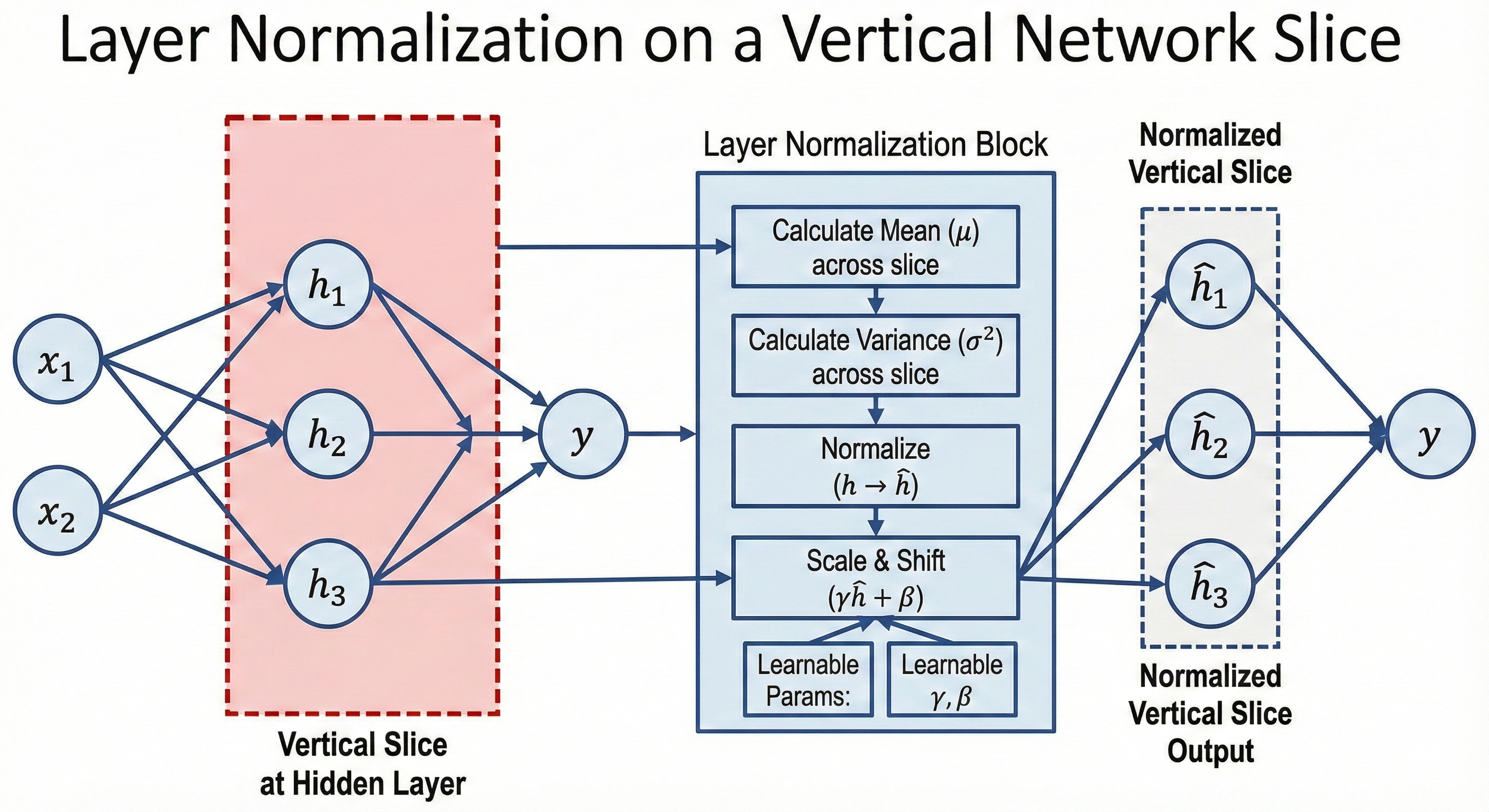
2. Mathematical Formulation and Derivation

Let $x$ be the input vector to the normalization layer for a single sample. Let $H$ be the number of hidden units (features) in that layer. $x = [x_1, x_2, …, x_H]$

The process involves four distinct steps:

Step A: Calculate Mean ($\mu$)

We calculate the mean across all hidden units for the single sample.

\[\mu = \frac{1}{H} \sum_{j=1}^{H} x_j\]

Step B: Calculate Variance ($\sigma^2$)

We calculate the variance across the same hidden units.

\[\sigma^2 = \frac{1}{H} \sum_{j=1}^{H} (x_j - \mu)^2\]

Step C: Normalize ($\hat{x}$)

We normalize the vector using the calculated statistics. We add a small constant $\epsilon$ (epsilon) to the denominator for numerical stability (to prevent division by zero).

\[\hat{x}_j = \frac{x_j - \mu}{\sqrt{\sigma^2 + \epsilon}}\]

Step D: Scale and Shift ($y$)

To ensure the transformation represents the identity function if necessary (preserving the network’s expressive power), we introduce two learnable parameters:

• $\gamma$ (Gamma): Scaling parameter
• $\beta$ (Beta): Shifting parameter

\[y_j = \gamma \cdot \hat{x}_j + \beta\]

3. Training vs. Inference Phase

A key distinction between LayerNorm and BatchNorm is how statistics and parameters are handled during different phases.

How Parameters ($\gamma, \beta$) are Learnt

• Initialization: Typically, $\gamma$ is initialized to vectors of $1$s, and $\beta$ is initialized to vectors of $0$s.
• Training: During backpropagation, the gradients with respect to $\gamma$ and $\beta$ are computed based on the loss function. These parameters are updated by the optimizer (e.g., Adam, SGD) just like weights and biases.

Usage in Training Phase

• For every input sample, $\mu$ and $\sigma$ are calculated dynamically based on the current values of the hidden units.
• The normalization is applied immediately.

Usage in Inference Phase (Crucial Difference)

Unlike Batch Normalization, which uses “running averages” (global statistics) calculated during training for inference:

• Layer Normalization does NOT use running averages.
• Because LayerNorm depends only on the current sample, $\mu$ and $\sigma$ are computed on the fly for every single prediction input during inference.
• This simplifies the deployment pipeline, as you do not need to carry over statistical buffers from the training state.

4. Practical Example with Numbers

Let’s assume we have a single input sample with 3 features (Hidden size $H=3$). We will assume $\epsilon \approx 0$ for simplicity.

Input Vector: $x = [2, 4, 12]$ Learnable Params: $\gamma = [1, 1, 1]$, $\beta = [3, 3, 3]$ (Initialized to 3 for this example).

Step 1: Compute Mean

\[\mu = \frac{2 + 4 + 12}{3} = \frac{18}{3} = 6\]

Step 2: Compute Variance

\[\sigma^2 = \frac{(2-6)^2 + (4-6)^2 + (12-6)^2}{3}\] \[\sigma^2 = \frac{(-4)^2 + (-2)^2 + (6)^2}{3}\] \[\sigma^2 = \frac{16 + 4 + 36}{3} = \frac{56}{3} \approx 18.67\]

Standard Deviation $\sigma = \sqrt{18.67} \approx 4.32$

Step 3: Normalize ($\hat{x}$)

• Feature 1: $(2 - 6) / 4.32 = -0.92$
• Feature 2: $(4 - 6) / 4.32 = -0.46$
• Feature 3: $(12 - 6) / 4.32 = 1.39$

Normalized Vector $\hat{x} \approx [-0.92, -0.46, 1.39]$

Step 4: Scale and Shift ($y$)

We apply $y = \gamma \hat{x} + \beta$. Since $\gamma=1$ and $\beta=3$:

• Feature 1: $(1 \cdot -0.92) + 3 = 2.08$
• Feature 2: $(1 \cdot -0.46) + 3 = 2.54$
• Feature 3: $(1 \cdot 1.39) + 3 = 4.39$

Final Output: $[2.08, 2.54, 4.39]$

The diverse input range $[2, 12]$ has been constrained to a stable range closer to the learnable beta, stabilizing the gradients for the next layer.