The Wisdom of Trees, Part 1: Decision Trees

The Wisdom of Trees series: Part 1: Decision Trees · Part 2: Random Forests

Imagine playing a game of “20 Questions.” We are trying to guess an object, and we can only ask yes/no questions. To win quickly, we wouldn’t ask, “Is it a 1994 Ford Taurus?” right away. We’d ask broad questions to narrow down the possibilities efficiently: “Is it alive?”, “Is it bigger than a breadbox?”

A Decision Tree is essentially a machine learning algorithm playing an optimized version of “20 Questions” with our data.

1. High-Level Definition and CART

At a high level, a decision tree is a supervised learning algorithm used for both classification (predicting a category, like “Watch” or “Skip”) and regression (predicting a number, like a movie rating).

It works by breaking down a dataset into smaller and smaller subsets while at the same time an associated decision tree is incrementally developed. The final result is a tree with decision nodes and leaf nodes. A decision node (e.g., “Is the lead actor Ryan Reynolds?”) has two or more branches, representing values for the attribute tested. Leaf node (e.g., “Watch”) represents a final decision or prediction.

The Standard: CART (Classification and Regression Trees)

While there are several types of decision trees (like ID3 or C4.5), the modern standard implemented in most libraries (like Python’s scikit-learn) is the CART algorithm.

Crucially, CART trees create binary splits. This means every question must have exactly two answers (Yes/No, True/False, or Less than/Greater than). Even if a category has three options (e.g., Action, Comedy, Drama), CART won’t split it three ways at once.

Two clarifications matter here, because they are a common source of confusion. First, a binary categorical split is not limited to “one category versus all others.” In principle CART can compare any subset of categories against its complement (with $k$ categories there are $2^{k-1}-1$ nontrivial partitions), and some libraries implement exactly that. Second, and more practically: scikit-learn’s trees do not consume categorical strings at all. They require numeric input, so “Action, Comedy, Drama” must be encoded first - typically one-hot (each category becomes its own “is-it-Action?” indicator, exposing category-versus-rest splits) or ordinal (which imposes an artificial order the tree treats as numeric). The clean mental model for scikit-learn is therefore: encode categoricals to numbers, after which every split is a threshold on one numeric column.

2. The Dataset: The Movie Night Dilemma

To understand the math, we need data. Let’s try to predict two things: whether we will Watch a movie (Classification) and what Rating (out of 10) we might give it (Regression).

Here is our dataset of 15 movies:

Movie ID	Lead Actor	Genre	Duration (mins)	Target 1: Watched? (Class)	Target 2: Rating (Reg)
1	Ryan Reynolds	Comedy	95	Yes	8.5
2	Ryan Reynolds	Action	110	Yes	8.0
3	Ryan Reynolds	Comedy	105	Yes	9.0
4	Ryan Reynolds	Drama	130	No	6.5
5	Ryan Reynolds	Action	125	Yes	7.5
6	Meryl Streep	Drama	140	Yes	9.5
7	Meryl Streep	Drama	160	Yes	9.0
8	Meryl Streep	Comedy	110	No	7.0
9	Meryl Streep	Drama	135	Yes	8.5
10	Meryl Streep	Action	120	No	6.0
11	Keanu Reeves	Action	115	Yes	8.5
12	Keanu Reeves	Sci-Fi	150	Yes	9.0
13	Keanu Reeves	Sci-Fi	100	Yes	8.0
14	Keanu Reeves	Drama	145	No	5.5
15	Keanu Reeves	Action	135	No	7.0

Summary Stats:

• Total Samples ($N$): 15
• Watched = Yes: 10 ($p_{yes} = 10/15 = 2/3 \approx 0.667$)
• Watched = No: 5 ($p_{no} = 5/15 = 1/3 \approx 0.333$)

(The counts break down as Reynolds 4 Yes / 1 No, Streep 3 Yes / 2 No, Reeves 3 Yes / 2 No.)

3. The Algorithm Step-by-Step (Defining the Math)

The core idea of decision tree building is greedy recursive partitioning.

• Greedy: At each step, pick the single best split right now, without worrying about future steps.
• Recursive Partitioning: Take a dataset, split it into two based on a rule, then repeat the process on the two resulting smaller datasets.

The goal is to create “pure” leaf nodes. For classification, a pure node contains only one class (e.g., 100% “Yes”). For regression, a pure node contains values that are all very close to each other (low variance).

How do we measure “purity”? We measure the opposite: Impurity.

Classification Metrics: Entropy and Gini

For a node $S$ with classes $i=1$ to $C$, where $p_i$ is the proportion of items belonging to class $i$:

1. Entropy (A measure of disorder/uncertainty) A classic concept from information theory. It ranges from 0 (perfectly pure) to $\log_2(C)$ (maximum disorder). For a binary classification (Yes/No), max entropy is 1 (a 50/50 split).

\[Entropy(S) = - \sum_{i=1}^{C} p_i \log_2(p_i)\]

Note: By convention, $0 \log_2(0) = 0$.

2. Gini Impurity (Probability of misclassification) A measure of how often a randomly chosen element from the set would be incorrectly labeled if it were randomly labeled according to the distribution of labels in the subset. It ranges from 0 (perfectly pure) to 0.5 (maximum impurity for binary classification). It’s generally faster to compute than log-based entropy.

\[Gini(S) = 1 - \sum_{i=1}^{C} (p_i)^2\]

3. Information Gain (The Deciding Factor) To decide which feature to split on, we calculate the potential Information Gain (IG). IG is simply the impurity of the parent node minus the weighted average impurity of the child nodes created by the split. We want the split that maximizes IG.

\[\Delta I = I(\text{Parent}) - \left[ \frac{N_{Left}}{N_{Parent}} I(\text{Left}) + \frac{N_{Right}}{N_{Parent}} I(\text{Right}) \right]\]

A note on names: strictly, information gain is this quantity when the impurity $I$ is entropy. When $I$ is Gini or (for regression) variance, the neutral term is impurity decrease or criterion reduction, and that is what we report below. The mechanic - parent impurity minus the weighted child impurity - is identical either way.

Regression Metric: Variance Reduction

For regression, we can’t use classes. Instead, we want the numerical values in a node to be clustered tightly around the average. We use Variance (or Mean Squared Error - MSE) as our measure of impurity.

\[Variance(S) = \frac{1}{N} \sum_{j=1}^{N} (y_j - \bar{y})^2\]

Where $y_j$ is an individual target value and $\bar{y}$ is the mean of values in that node.

The goal in regression is to maximize Variance Reduction, calculated exactly the same way as Information Gain above, just replacing entropy/gini with variance.

4. Running the Algorithm (Exact Calculations)

Let’s build the first node of our classification tree (Target: “Watched?”). We need to find the best split among Actor, Genre, and Duration.

Step 0: Calculate Baseline Impurity of the Whole Dataset (Parent Node)

• 10 Yes, 5 No ($p_{yes}=2/3, p_{no}=1/3$)
• Base Entropy: $- (\tfrac{2}{3} \log_2 \tfrac{2}{3} + \tfrac{1}{3} \log_2 \tfrac{1}{3}) \approx -(-0.390 - 0.528) = \textbf{0.918}$
• Base Gini: $1 - ((2/3)^2 + (1/3)^2) = 1 - (0.444 + 0.111) = \textbf{0.444}$

Candidate Split 1: Categorical Feature (Lead Actor)

CART needs a binary split. Let’s test: “Is Lead Actor == Ryan Reynolds?”

• Left Child (True - Reynolds): Total 5 movies.
  • Watched: 4 Yes, 1 No ($p_{yes}=0.8, p_{no}=0.2$)
• Right Child (False - Not Reynolds): Total 10 movies (Streep + Reeves).
  • Watched: 6 Yes, 4 No ($p_{yes}=0.6, p_{no}=0.4$)

Calculation using Entropy:

1. Entropy(Left): $- (0.8 \log_2 0.8 + 0.2 \log_2 0.2) \approx \textbf{0.722}$
2. Entropy(Right): $- (0.6 \log_2 0.6 + 0.4 \log_2 0.4) \approx \textbf{0.971}$
3. Weighted Impurity of Children: $(\frac{5}{15} \times 0.722) + (\frac{10}{15} \times 0.971) = 0.241 + 0.647 = \textbf{0.888}$
4. Information Gain (Entropy): $0.918 (\text{Base}) - 0.888 (\text{Children}) = \textbf{0.030}$

Calculation using Gini Impurity:

1. Gini(Left): $1 - (0.8^2 + 0.2^2) = 1 - (0.64 + 0.04) = \textbf{0.32}$
2. Gini(Right): $1 - (0.6^2 + 0.4^2) = 1 - (0.36 + 0.16) = \textbf{0.48}$
3. Weighted Impurity of Children: $(\frac{5}{15} \times 0.32) + (\frac{10}{15} \times 0.48) = 0.107 + 0.320 = \textbf{0.427}$
4. Gini Decrease: $0.444 (\text{Base}) - 0.427 (\text{Children}) = \textbf{0.018}$

We would repeat this for “Actor == Streep” and “Actor == Reeves” to find the best Actor split.

Candidate Split 2: Numerical Feature (Duration)

How does a tree split continuous numbers like duration? It tests “thresholds.”

1. Sort the unique durations: 95, 100, 105, 110, 115, 120, 125, 130, 135, 140, 145, 150, 160.
2. Use the midpoints between values as candidate splits: 97.5, 102.5, 107.5, etc.

Let’s test the split: “Duration < 117.5?” (Midpoint between 115 and 120).

• Left Child (Duration < 117.5): Movies 1, 2, 3, 8, 11, 13. Total 6 movies.
  • Watched: 5 Yes, 1 No ($p_{yes} \approx 0.83, p_{no} \approx 0.17$)
• Right Child (Duration >= 117.5): The remaining 9 movies.
  • Watched: 5 Yes, 4 No ($p_{yes} \approx 0.56, p_{no} \approx 0.44$)

Let’s calculate the Gini decrease for this split:

1. Gini(Left): $1 - ((5/6)^2 + (1/6)^2) = 1 - (0.694 + 0.028) = \textbf{0.278}$
2. Gini(Right): $1 - ((5/9)^2 + (4/9)^2) = 1 - (0.309 + 0.198) = \textbf{0.494}$
3. Weighted Impurity: $(\frac{6}{15} \times 0.278) + (\frac{9}{15} \times 0.494) = 0.111 + 0.296 = \textbf{0.407}$
4. Gini Decrease: $0.444 (\text{Base}) - 0.407 (\text{Children}) = \textbf{0.037}$

The Winner and Full Tree Construction

The two splits we worked by hand give Gini decreases of 0.018 (Actor == Reynolds) and 0.037 (Duration < 117.5), so duration is ahead. But the greedy algorithm does not stop at two candidates: it evaluates every binary actor split, every genre split, and every duration threshold, then keeps the single largest decrease. Here are the best of each kind:

Candidate split	Left (Y/N)	Right (Y/N)	Gini decrease
Duration < 107.5	3 / 0	7 / 5	0.0556
Duration < 117.5	5 / 1	5 / 4	0.0370
Genre == Sci-Fi	2 / 0	8 / 5	0.0342
Actor == Reynolds	4 / 1	6 / 4	0.0178

The winner is Duration < 107.5, not the 117.5 split we happened to try first. It carves off a perfectly pure group (movies 1, 3, 13: three shorter films, all Watched) and leaves a 7-Yes / 5-No remainder to split further. This is worth pausing on: the “obvious” threshold near the middle of the range is not the best one, which is exactly why the algorithm searches exhaustively rather than guessing. Running scikit-learn on this dataset picks the same root, Duration <= 107.5.

Continuing greedily on the 12-movie right child, the next best split is Duration < 147.5:

• Node 1 (Root): Duration < 107.5?
  • True (3 movies): all Watched - a pure leaf that predicts “Yes”.
  • False (12 movies): Duration < 147.5?
    • True (10 movies): a 5-Yes / 5-No node the tree keeps splitting (or turns into a majority leaf if a depth limit stops it).
    • False (2 movies): both Watched - a pure “Yes” leaf.

The process stops when a node is 100% pure, or we hit a predefined limit (like maximum depth).

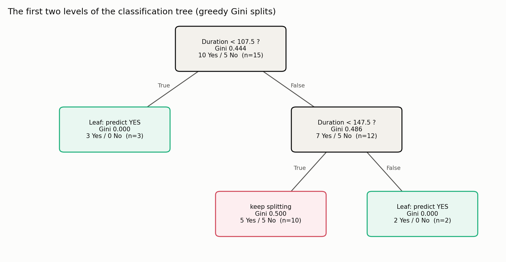
Each box shows the split question, the node’s Gini, and its class counts. Notice how impurity falls from 0.444 at the root toward 0 in the pure leaves - that drop, weighted by node size, is exactly the impurity decrease the algorithm maximizes.

A Regression Split on the Same Data

The identical machinery builds a regression tree for the Rating target; we simply swap Gini for variance. The whole dataset has mean rating $\bar{y} \approx 7.83$ and variance $\approx 1.356$. Score the very same Duration < 107.5 split:

• Left (movies 1, 3, 13): ratings 8.5, 9.0, 8.0. Mean 8.5, variance $\approx 0.167$.
• Right (12 movies): mean $\approx 7.67$, variance $\approx 1.514$.
• Weighted variance: $\frac{3}{15}(0.167) + \frac{12}{15}(1.514) \approx 1.244$.
• Variance reduction: $1.356 - 1.244 \approx 0.111$.

One subtlety is worth flagging: the criterion changes the tree. For the Rating target the greedy search actually prefers Duration < 147.5 (variance reduction $\approx 0.209$), which isolates the two longest, highest-rated films. The best classification split (107.5) and the best regression split (147.5) differ on the same data, because Gini and variance reward different groupings.

5. Inference: Making Predictions

We have a trained tree. A new movie arrives: Keanu Reeves, Sci-Fi, Duration 100.

Classification Inference (“Watched?”) We drop the movie down the tree:

1. Is Duration < 107.5? Yes (100 < 107.5). Go to the left leaf.
2. That leaf holds the three short training films (movies 1, 3, 13), all Watched.

• Pure leaf: here the leaf is [3 Yes, 0 No], so the prediction is “Yes” with $P(\text{Yes}) = 3/3 = 100\%$.
• Impure leaf (in general): had the leaf held [4 Yes, 1 No], the prediction would be the majority class “Yes”, with probability $P(\text{Yes}) = 4/5 = 80\%$.

Regression Inference (“Rating”) The traversal is identical; only the leaf summary changes. That same left leaf holds ratings [8.5, 9.0, 8.0], so a regression tree predicts their average: $(8.5 + 9.0 + 8.0)/3 = \textbf{8.5}$.

6. Overfitting: The Curse of the Decision Tree

Decision trees are notorious for overfitting. Why? Because they are “non-parametric” and can grow indefinitely complex. If allowed, a tree keeps splitting until its leaves are pure or can no longer be split.

A fully grown tree can drive training error very low and, in doing so, fit the noise rather than the signal. (It is not guaranteed to hit exactly 0% - duplicate feature vectors with conflicting labels, sample weights, or exhausted splits can leave impure leaves.) The real danger is high variance: such a tree swings sharply with small data changes and can generalize poorly to new movies. Overfitting is a risk to measure on held-out data, not an automatic verdict on every deep tree.

How to Prevent Overfitting

We prevent this using Regularization (constraints) or Pruning.

1. Pre-Pruning (Constraints during build time):

• Max Depth: Stop the tree from growing deeper than, say, 3 levels.
• Min Samples Split: Only allowed to split a node if it has at least, say, 5 samples.
• Min Samples Leaf: A split is only valid if the resulting left and right children both have at least, say, 3 samples.
• Max Leaf Nodes: Cap the total number of terminal nodes.

2. Post-Pruning (Cleaning up afterward): Grow the tree to its maximum extent, then cut back branches that add little predictive power. Cost-complexity pruning makes this precise by minimizing

\[R_\alpha(T) = R(T) + \alpha \lvert \widetilde{T} \rvert,\]

where $R(T)$ is the total impurity of the tree’s leaves and $\lvert \widetilde{T} \rvert$ is the number of leaves. The penalty $\alpha$ trades fit against size: $\alpha = 0$ keeps the full tree, larger $\alpha$ prunes more aggressively. The pruning path produces a sequence of candidate subtrees, and ccp_alpha should be chosen on validation or cross-validation data, never the final test set.

7. Decision Boundaries

How does a decision tree view the world?

Because every split is a hard binary threshold on a single feature (e.g., Duration < 107.5), decision trees create orthogonal, axis-parallel decision boundaries.

If we plotted “Duration” vs. another numerical feature, the decision boundary wouldn’t be a smooth curve or a diagonal line. It would look like a series of stairs or rectangular boxes.

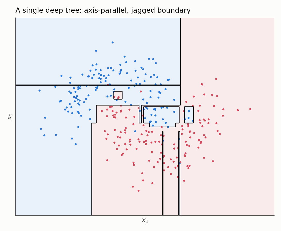
While individual boundaries are linear (straight lines), the combination of many such splits allows the tree to approximate highly non-linear relationships. The price of an unconstrained tree is visible in the little islands above: isolated boxes drawn around one or two noisy points, the signature of overfitting.

One boundary a tree cannot cross is the range of what it has seen. A leaf predicts a summary of its training targets (a majority class, or an average value), so a regression tree in our data can never output a rating above 9.5 or below 5.5: it does not extrapolate beyond the observed target range. That is a real limitation whenever the true relationship keeps climbing outside the training span.

8. Determining Variable Importance

One of the best features of decision trees is interpretability. We can measure how important each feature was.

Variable importance is calculated by summing up the Information Gain (or Variance Reduction) brought by a specific feature across all nodes where it was used to split.

If “Duration” was used three times in the tree, and those splits cleaned up the data significantly (high IG weighted by the number of samples involved), it will have high importance. These scores are usually normalized so they sum to 1 (or 100%).

In our movie example, if Duration splits consistently separated “Yes” from “No” better than Actor, Duration would have a higher variable importance score.

9. Handling Missing Data

What if we don’t know the duration of a movie?

The current scikit-learn reality: modern scikit-learn trees do handle missing values natively. DecisionTreeClassifier and DecisionTreeRegressor gained native NaN routing in version 1.3, and the random forests followed in 1.4 (with the default splitter='best' and the standard criteria). At each candidate split the learner evaluates whether the missing rows should go left or right, and stores the direction that helps most. The old advice that “scikit-learn cannot handle missing values” is simply out of date.

A few caveats still apply:

• Support depends on the estimator, its version, and dense-versus-sparse input, so confirm before relying on it.
• A missingness indicator (an extra 0/1 column flagging “was this absent?”) is worth adding when absence itself carries signal.
• A placeholder like -1 is unsafe unless it is a genuine, deliberately modeled value - a tree reads it as ordered numeric data and may split on it as though it were a real duration.

Other algorithms take different routes: C4.5 uses surrogate splits (fall back to the feature most correlated with the primary one), while gradient-boosted libraries such as XGBoost learn a default direction for missing values at each node.

10. Handling Imbalanced Datasets

What if our dataset had 14 “Yes” movies and only 1 “No”?

The problem is subtler than “the tree ignores the minority class.” A tree does have an impurity incentive to isolate a rare class whenever a feature offers a clean split for it. What actually goes wrong is that accuracy looks great (predict “Yes” for everything scores 93%), the absolute impurity gain from splitting off a single example is tiny, and constraints like min_samples_leaf or weak features can leave the lone “No” unsplit. Minority performance suffers even though the algorithm is not literally indifferent.

How to handle it:

1. Class or sample weights: class_weight tells the algorithm a minority mistake costs more (say 10x), reshaping the impurity math to prioritize the rare class.
2. The right metrics: stop reading plain accuracy. Use balanced accuracy, recall, F1, or PR-AUC, and tune the decision threshold on predicted probabilities.
3. Stratified validation: keep the class ratio consistent across cross-validation folds.
4. Resampling, carefully: undersample the majority or synthesize minority examples (e.g. SMOTE), but only inside the training folds to avoid leakage. Simply duplicating the single “No” thirteen times adds weight without new information and can deepen memorization - it is not a general fix.

---

A single tree is fast, readable, and - as we have seen - dangerously eager to overfit. That instability is not a dead end; it is the raw material for something sturdier. Part 2: Random Forests shows how averaging many deliberately decorrelated trees turns this high-variance learner into one of the most dependable tools for tabular data.

Resources

• Breiman, L., Friedman, J. H., Olshen, R. A., & Stone, C. J. (1984). Classification and Regression Trees. Wadsworth, Belmont, CA. (The original CART reference.)
• scikit-learn: Decision Trees - user guide, including the missing-value and categorical-encoding notes.