Boosting, Part 2: The XGBoost Mathematics
- Decision trees
- Random Forests
- AdaBoost and gradient boosting
- The XGBoost mathematics You are here
- Choosing a boosting library
Part 1 built gradient boosting as gradient descent in function space. XGBoost keeps that idea but rebuilds the objective: a regularized loss, a second-order (Newton) approximation, and a closed-form leaf value that doubles as a split criterion. This part is the full derivation, followed by the regression and classification specifics and how the equations map to real hyperparameters.
High-Level Motivation XGBoost was created to push the limits of computation and performance. It is a scalable end-to-end tree boosting system. Its key motivations are execution speed (via parallelization and cache optimization) and model performance (via a smarter regularized objective).
What XGBoost adds (design and engineering choices, not mathematics unavailable to other gradient boosters):
- Regularized objective: an explicit leaf-count penalty plus L2 (and optional L1) on leaf weights, folded directly into the split criterion.
- Second-order optimization: it uses the Hessian as well as the gradient. Newton-style boosting predates the library, but XGBoost made it the default and paired it with the regularized objective.
- Sparsity-aware split finding: a learned default direction for missing and sparse (e.g. one-hot) entries.
- Systems engineering: cache-aware block structures, out-of-core (disk-based) training, and parallel/distributed split finding.
Here is the complete step-by-step derivation of the XGBoost loss function optimization, specifically applied to a Regression problem.
1. The Objective Function
XGBoost aims to minimize a regularized objective function. For a model with $K$ trees, the objective is the sum of the loss function (how well we fit the data) and a regularization term (to control complexity).
\[\text{Obj} = \sum_{i=1}^n l(y_i, \hat{y}_i) + \sum_{k=1}^K \Omega(f_k)\]Where:
- $n$: Number of training examples.
- $l(y_i, \hat{y}_i)$: A differentiable convex loss function (e.g., Mean Squared Error for regression).
- $\Omega(f_k)$: Regularization term for tree $f_k$.
- $\Omega(f) = \gamma T + \frac{1}{2}\lambda \lVert w \rVert^2$.
- $T$: Number of leaves in the tree.
- $w$: Scores (weights) of the leaves.
- $\gamma, \lambda$: Regularization hyperparameters.
This derivation covers the leaf-count penalty and L2 only. XGBoost also supports an L1 term $\alpha \sum_j \lvert w_j \rvert$; to keep the algebra clean we set $\alpha = 0$ here. (With $\alpha > 0$ the leaf optimum below gains a soft-thresholding numerator, $w_j^\ast = -\operatorname{sgn}(G_j)\max(\lvert G_j\rvert - \alpha, 0) / (H_j + \lambda)$.)
2. Additive Training (Step-by-Step)
XGBoost trains systematically. At step $t$, we add a new tree $f_t(x_i)$ to the previous prediction $\hat{y}_i^{(t-1)}$ to minimize the new objective.
\[\text{Obj}^{(t)} = \sum_{i=1}^n l\left(y_i, \hat{y}_i^{(t-1)} + f_t(x_i)\right) + \Omega(f_t)\]3. Second-Order Taylor Expansion
This is the key innovation. Instead of using just the gradient (like traditional Gradient Boosting), XGBoost approximates the loss function using a second-order Taylor expansion around the current prediction $\hat{y}_i^{(t-1)}$.
Taylor Series Approximation:
\[f(x + \Delta x) \approx f(x) + f'(x)\,\Delta x + \frac{1}{2} f''(x)\,(\Delta x)^2\]Treating $\hat{y}_i^{(t-1)}$ (the prediction so far) as $x$ and $f_t(x_i)$ (the increment) as $\Delta x$, we get:
\[\text{Obj}^{(t)} \approx \sum_{i=1}^n \left[ l(y_i, \hat{y}_i^{(t-1)}) + g_i f_t(x_i) + \frac{1}{2}h_i f_t^2(x_i) \right] + \Omega(f_t)\]Where $g_i$ and $h_i$ are the first and second order gradients (derivatives) of the loss function with respect to the prediction:
- Gradient ($g_i$): $\partial_{\hat{y}^{(t-1)}} l(y_i, \hat{y}^{(t-1)})$
- Hessian ($h_i$): $\partial^2_{\hat{y}^{(t-1)}} l(y_i, \hat{y}^{(t-1)})$
Since $l(y_i, \hat{y}_i^{(t-1)})$ is constant at step $t$, we can remove it to get the simplified objective:
\[\text{Obj}^{(t)} \approx \sum_{i=1}^n \left[ g_i f_t(x_i) + \frac{1}{2}h_i f_t^2(x_i) \right] + \Omega(f_t)\]4. Regression Specifics: Deriving $g_i$ and $h_i$
For a Regression problem, we typically use the Mean Squared Error (MSE) loss:
\[l(y, \hat{y}) = \frac{1}{2}(y - \hat{y})^2\]Let’s derive $g_i$ and $h_i$ for this specific loss:
First Derivative ($g_i$):
\[g_i = \frac{\partial}{\partial \hat{y}} \left( \frac{1}{2}(y - \hat{y})^2 \right) = \frac{\partial}{\partial \hat{y}} \left( \frac{1}{2}(y^2 - 2y\hat{y} + \hat{y}^2) \right) = -(y - \hat{y}) = \hat{y} - y\]Second Derivative ($h_i$):
\[h_i = \frac{\partial}{\partial \hat{y}} (\hat{y} - y) = 1\]
So for MSE regression, $g_i = \hat{y} - y$ is the negative of the conventional residual $y - \hat{y}$ (a gradient points uphill), and $h_i$ is constant (1). The minus sign in the leaf-weight formula below flips it back, which is why the optimal leaf value comes out as the mean residual.
5. Grouping by Leaves
Now, we define the tree $f_t(x)$ by its leaf weights. If a data point $x_i$ falls into leaf $j$, then $f_t(x_i) = w_j$. We can rewrite the sum over data points ($n$) as a sum over leaves ($T$). Let $I_j$ be the set of data points in leaf $j$.
Expanding the regularization term $\Omega(f_t) = \gamma T + \frac{1}{2}\lambda \sum_{j=1}^T w_j^2$:
\[\text{Obj}^{(t)} = \sum_{j=1}^T \left[ \left( \sum_{i \in I_j} g_i \right) w_j + \frac{1}{2} \left( \sum_{i \in I_j} h_i + \lambda \right) w_j^2 \right] + \gamma T\]6. Finding the Optimal Leaf Weights ($w_j^\ast$)
To find the optimal weight for leaf $j$, we take the derivative of the objective with respect to $w_j$ and set it to zero.
\[\frac{\partial \text{Obj}}{\partial w_j} = \sum_{i \in I_j} g_i + \left( \sum_{i \in I_j} h_i + \lambda \right) w_j = 0\]Solving for $w_j$:
\[w_j^* = - \frac{\sum_{i \in I_j} g_i}{\sum_{i \in I_j} h_i + \lambda}\]For our Regression case (where $h_i=1$):
\[w_j^* = - \frac{\sum ( \hat{y} - y )}{N_j + \lambda} = \frac{\sum ( y - \hat{y} )}{N_j + \lambda}\]This means the optimal leaf value is simply the average of residuals in that leaf (regularized). Note that with $\lambda > 0$ it is not exactly the average: it is the residual sum divided by $N_j + \lambda$, a shrunk mean.
Shrinkage. The closed form $w_j^\ast$ is the unshrunken optimum of the local quadratic. In practice XGBoost scales each new tree’s contribution by a learning rate $\eta$ before adding it:
\[\hat{y}_i^{(t)} = \hat{y}_i^{(t-1)} + \eta\, f_t(x_i).\]Omitting $\eta$ would make the math disagree with the regularization discussion and with how the model actually trains.
7. The Optimal Loss Value (Structure Score)
Finally, we substitute the optimal weight $w_j^\ast$ back into the objective function to get the minimum possible loss for a given tree structure. This is used as the Structure Score to evaluate split candidates.
\[\text{Score} = - \frac{1}{2} \sum_{j=1}^T \frac{(\sum_{i \in I_j} g_i)^2}{\sum_{i \in I_j} h_i + \lambda} + \gamma T\]Two sign conventions float around here, so it helps to pin them down. The formula above is the minimized objective: it is negative (lower is better), and it equals the true objective only up to the constant loss term we dropped and the Taylor approximation. Most write-ups instead quote a positive quality score (often called the “similarity score”), $\frac{1}{2}\frac{(\sum_{i} g_i)^2}{\sum_{i} h_i + \lambda}$ per leaf, where higher is better. These are the same quantity with opposite signs. Split selection uses the positive version: XGBoost picks the split that maximizes the Gain, the combined quality of the two children minus the parent, minus the per-split penalty $\gamma$:
\[\text{Gain} = \frac{1}{2} \left[ \frac{G_L^2}{H_L+\lambda} + \frac{G_R^2}{H_R+\lambda} - \frac{(G_L+G_R)^2}{H_L+H_R+\lambda} \right] - \gamma\]Where $G = \sum g_i$ and $H = \sum h_i$ for Left (L) and Right (R) children.
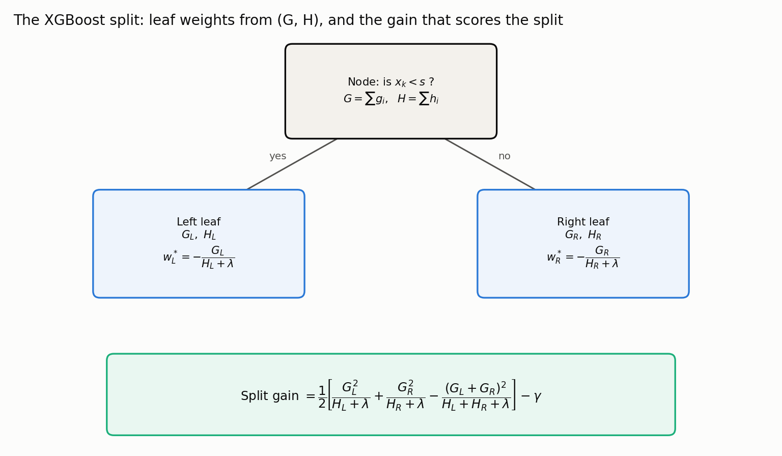
Every piece of the derivation lives in this one picture: each leaf’s optimal weight $w^\ast$ comes from its $(G, H)$, and the split is chosen to maximize the gain, the combined leaf quality of the children minus the parent, minus the per-split penalty $\gamma$.
8. Regression vs. Classification, and Missing Values
4. Table: Regression vs. Classification Formulae Here is how the general $g_i$ and $h_i$ translate to specific tasks (deriving from the general formulae above):
| Component | Regression (MSE Loss) | Classification (Log Loss) |
|---|---|---|
| Gradient ($g_i$) | $\hat{y}_i - y_i$ | $p_i - y_i$ |
| Hessian ($h_i$) | $1$ (Constant) | $p_i(1 - p_i)$ |
| Similarity Score | $\frac{(\sum(\hat{y}_i - y_i))^2}{N_{leaf} + \lambda}$ | $\frac{(\sum (p_i - y_i))^2}{\sum p_i(1-p_i) + \lambda}$ |
| Leaf Output (Weight) | $\frac{\sum(y_i - \hat{y}_i)}{N_{leaf} + \lambda}$ | $\frac{\sum (y_i - p_i)}{\sum p_i(1-p_i) + \lambda}$ |
(Note: $\lambda$ is the L2 regularization parameter).
5. Handling Missing Features XGBoost uses a Sparsity-aware Split Finding algorithm. It does not impute missing values. Instead, during training, it tests placing all missing values into the Left child and calculates the gain. Then it tests placing them in the Right child. It learns the optimal default direction for missing data for every single split in the tree.
With the objective, leaf weights, and split gain in hand, the remaining question is which implementation to reach for. Part 3: Choosing a Library compares XGBoost, LightGBM, and CatBoost on the dimensions that actually differ.
Resources
- Chen, T. & Guestrin, C. (2016). XGBoost: A Scalable Tree Boosting System. KDD ‘16, 785-794.
- XGBoost parameter documentation - the practical names behind the math:
eta,gamma,lambda,alpha,min_child_weight,max_depth.