The Wisdom of Trees, Part 2: Random Forests

Posted Nov 21, 2025

By Sayan Biswas

14 min read

The Wisdom of Trees series: Part 1: Decision Trees · Part 2: Random Forests

In Part 1 we built a single Decision Tree - and saw how readily it overfits. That sets up a natural thought: “If one tree is good, surely a whole forest is better?”

That intuition is absolutely right. Welcome to the Random Forest.

1. Motivation: The Wisdom of Crowds

We established that a single Decision Tree is prone to overfitting. It’s like asking one highly opinionated friend for a movie recommendation. They might know our taste, but they might also be obsessed with obscure French cinema and lead us astray.

A Random Forest is the machine learning equivalent of asking 100 friends for a recommendation and going with the majority vote. While one friend might be biased or wrong, the “wisdom of the crowd” usually converges on the correct answer.

By combining many individual trees, we create a model that is more robust, stable, and accurate than any single constituent tree.

2. Ensemble, Bagging, and The Bias/Variance Trade-off

Random Forest is an Ensemble technique, meaning it combines multiple models to produce a single prediction. Specifically, it relies on a concept called Bagging.

What is Bagging?

Bagging stands for Bootstrap Aggregating. It involves two steps:

Bootstrapping: Creating many random subsets of the training data (sampling with replacement).
Aggregating: Training a separate model on each subset and combining their predictions.

The Math of Bias and Variance

Single Decision Tree: Has Low Bias (it can model complex patterns) but High Variance (it changes drastically with small data changes).
Random Forest: Maintains the Low Bias of the individual trees but significantly Reduces Variance.

Mathematically, if we average $B$ predictors each with variance $\sigma^2$ and equal pairwise correlation $\rho$, the variance of their average is:

\[\operatorname{Var}(\bar{T}) = \rho\,\sigma^2 + \frac{1 - \rho}{B}\,\sigma^2.\]

The independent case ($\rho = 0$) recovers the familiar $\sigma^2 / B$, but real forest trees are correlated: they share overlapping bootstrap samples and the same strong features keep resurfacing. This one equation explains the entire design of a Random Forest:

Adding trees (larger $B$) shrinks only the second term, the uncorrelated part of the variance.
The first term, $\rho\,\sigma^2$, is a floor that more trees cannot average away.
To lower that floor we must reduce $\rho$ - which is exactly what feature subsampling (next section) does, by stopping every tree from splitting on the same dominant feature.

There is a tension: forcing trees apart can weaken each individual tree, so the design trades tree strength against tree correlation. Breiman’s original analysis frames a forest’s generalization in precisely those two terms.

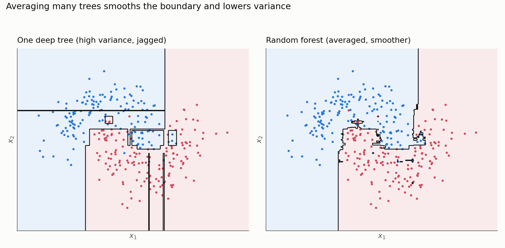
The contrast is the whole point. The single tree (left) draws a jagged boundary and fences off little islands around individual noisy points - high variance. The forest (right), averaging 300 such trees, keeps the same broad shape but smooths away the slivers. The bias stays low; the variance drops.

3. The Training Algorithm: Controlling the Chaos

A Random Forest is not just “Bagging trees.” It adds a second layer of randomness to ensure the trees are diverse. If we just bagged trees, they would all likely split on the strongest feature (e.g., “Lead Actor”) at the root, making them highly correlated.

To fix this, Random Forest modifies the tree-growing algorithm:

The Algorithm

Given a training set $D$ with $N$ samples and $P$ features, and a desired number of trees $B$:

For $b = 1$ to $B$:

Bootstrap Sample: Draw a sample $D_b$ of size $N$ from $D$ with replacement.
Grow Tree $T_b$: Grow a decision tree on $D_b$. However, at each node split:
- Do not look at all $P$ features.
- Select a random subset of $m$ features, where $m < P$.
- Find the best split only among these $m$ features.
- Split the node.
- Repeat until the tree is fully grown (no pruning is usually applied).

Choosing $m$ (Max Features)

Restricting the features per split is the “secret sauce” that lowers $\rho$. A fresh random subset of $m$ features is drawn at every node, not once per tree. Two figures are often quoted:

Classification: $m \approx \sqrt{P}$
Regression: $m \approx P/3$

Treat these as historical heuristics, not universal rules - and note they are not the current scikit-learn defaults, which are max_features="sqrt" for RandomForestClassifier and max_features=1.0 (all features) for RandomForestRegressor. When performance matters, tune $m$ jointly with min_samples_leaf, max_depth, max_samples, and the number of trees. Too small an $m$ weakens each tree (more bias); too large fails to decorrelate them.

4. Inference: Making Predictions

Once we have trained our forest of trees $\{T_1, T_2, …, T_B\}$, inference is simply an aggregation process. Let $x$ be a new input vector (a new movie).

For Regression

We take the average of the predictions from all individual trees.

\[\hat{y} = \frac{1}{B} \sum_{b=1}^{B} T_b(x)\]

For Classification

We can use “Hard Voting” or “Soft Voting.”

Hard Voting (Majority Vote): Let $C_b(x)$ be the class predicted by tree $b$.
\[\hat{y} = \text{mode} \{ C_1(x), C_2(x), ..., C_B(x) \}\]
Soft Voting (Averaged Probabilities): This is generally preferred. Let $p_b(c \vert x)$ be the probability that tree $b$ assigns to class $c$. We average the probabilities across all trees and pick the class with the highest average.
\[\hat{y} = \operatorname*{argmax}_c \left( \frac{1}{B} \sum_{b=1}^{B} p_b(c|x) \right)\]

Breiman’s original forest used hard tree votes; scikit-learn’s RandomForestClassifier uses soft voting - it averages the per-tree class probabilities and takes the argmax. One caution: a tree’s leaf-frequency probabilities, and their forest average, are not automatically calibrated. If we need trustworthy probabilities and not just the right class, we should evaluate calibration and, if necessary, fit a calibration step on separate data.

5. Bootstrapping and Out-of-Bag (OOB) Score

When we create a bootstrap sample of size $N$ from a dataset of size $N$ with replacement, statistically, about 36.8% of the unique rows are left out.

The Setup: Imagine a dataset with $N$ rows. To create a bootstrap sample for one tree, we draw $N$ times from this dataset with replacement.

Probability of being picked: The probability of picking a specific row (let’s call it Row $i$) in a single draw is $\frac{1}{N}$.
Probability of NOT being picked: Conversely, the probability of not picking Row $i$ in a single draw is $1 - \frac{1}{N}$.
Probability of NOT being picked in $N$ draws: Since the draws are independent, we multiply the probability $N$ times:
\[P(\text{Row } i \text{ is OOB}) = \left(1 - \frac{1}{N}\right)^N\]

The Limit: We want to know what this probability approaches as our dataset size ($N$) grows large. This brings us to a fundamental limit in calculus related to Euler’s number ($e$).

Recall the definition of $e$:

\[\lim_{N \to \infty} \left(1 + \frac{1}{N}\right)^N = e \approx 2.718\]

Our equation is slightly different (it has a minus sign), which converges to the inverse of $e$:

\[\lim_{N \to \infty} \left(1 - \frac{1}{N}\right)^N = \frac{1}{e} \approx \frac{1}{2.718} \approx \mathbf{0.368}\]

These left-out rows are called Out-of-Bag (OOB) samples.

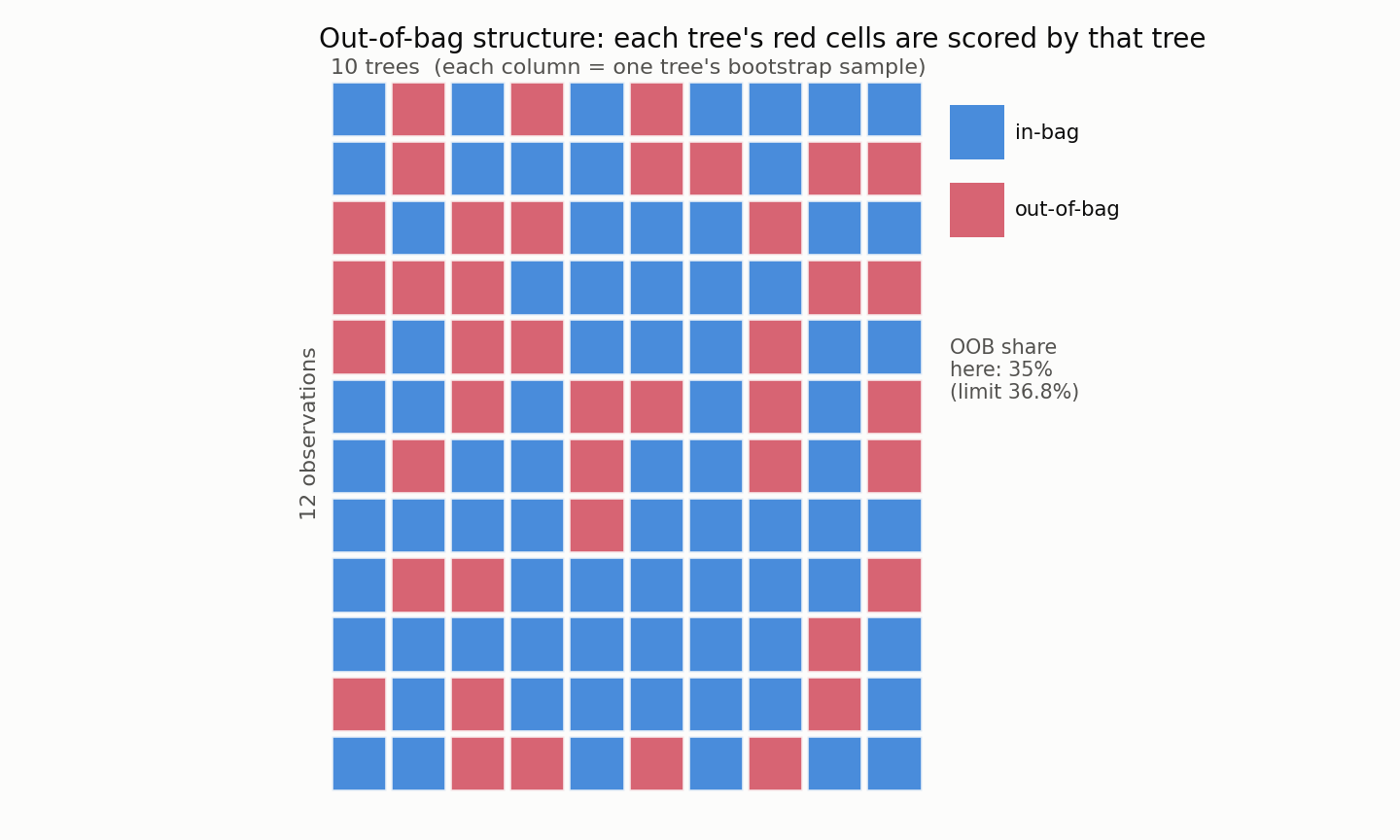
Read the grid by column: each tree’s bootstrap sample leaves roughly a third of the rows out (the red cells), and those are the rows that tree is allowed to score. Read it by row instead, and every observation is out-of-bag for several trees - exactly the trees we use to predict it.

This gives us a built-in generalization estimate. For every specific row in our dataset, there are several trees in the forest that never saw that row during training. We can push that row down only those specific trees to get a prediction.

The OOB Score aggregates the accuracy (or $R^2$) of these predictions across all rows. It is a convenient internal proxy for cross-validation, but it is an estimate, not a substitute for a final test set: repeatedly tuning against OOB can overfit it, row-wise bootstrapping ignores groups and time order, and OOB accuracy is uninformative under severe class imbalance. With too few trees, some rows also receive very few OOB votes. For a high-stakes claim, keep a genuinely untouched evaluation set.

6. Feature Importance Beyond Impurity: Permutation

Summing impurity decrease across splits (the previous section) is one way to rank features, but it has known biases we will note shortly. A complementary idea is permutation importance: if a feature matters, randomly shuffling its column should hurt the model’s predictions.

There are two distinct procedures here, and they are easy to conflate:

Breiman-style OOB permutation importance. For each tree, score its own OOB rows, then permute one feature within those OOB rows and measure how much that tree’s error rises. Average the increase across all trees. This one is internal to the forest.
Model-agnostic held-out permutation importance. Score the whole fitted model once on a validation or test set, permute one feature in that set, and measure the metric drop; repeat per feature. This works for any model - it is what scikit-learn’s permutation_importance computes on whatever dataset we hand it. It is not an automatic OOB method.

Both share the same logic and differ only in which data the shuffling happens on. The toy below illustrates the mechanic on a single tree’s OOB rows (procedure 1). To keep it concrete we use two features: the real signal “Lead Actor” and an injected noise column “Day of Week.”

The Scenario: We look at one tree, Tree #1, whose OOB set is 4 movies. The tree learned to predict from “Lead Actor” and ignores “Day of Week.”

Baseline Performance:

OOB Data:
1. [Reynolds, Monday] -> Watched (Tree Predicts: Watched) ✅
2. [Reynolds, Friday] -> Watched (Tree Predicts: Watched) ✅
3. [Streep, Tuesday] -> Skip (Tree Predicts: Skip) ✅
4. [Streep, Friday] -> Skip (Tree Predicts: Skip) ✅
Baseline Accuracy: 4/4 = 100%

Test 1: Check Importance of “Lead Actor” We shuffle the “Lead Actor” column randomly in the OOB data. The “Day of Week” stays the same.

Shuffled Data:
1. [Streep, Monday] -> Truth is Watched. Tree sees Streep, Predicts: Skip. ❌
2. [Reynolds, Friday] -> Truth is Watched. Tree sees Reynolds, Predicts: Watched. ✅
3. [Reynolds, Tuesday] -> Truth is Skip. Tree sees Reynolds, Predicts: Watched. ❌
4. [Streep, Friday] -> Truth is Skip. Tree sees Streep, Predicts: Skip. ✅
New Accuracy: 2/4 = 50%
Importance Score: $100\% - 50\% = \mathbf{50\%}$ (Huge Drop = High Importance)

Test 2: Check Importance of “Day of Week” We reset the data and this time shuffle the “Day of Week” column.

Shuffled Data:
1. [Reynolds, Friday] -> Truth is Watched. Tree sees Reynolds, Predicts: Watched. ✅
2. [Reynolds, Tuesday] -> Truth is Watched. Tree sees Reynolds, Predicts: Watched. ✅
3. [Streep, Monday] -> Truth is Skip. Tree sees Streep, Predicts: Skip. ✅
4. [Streep, Friday] -> Truth is Skip. Tree sees Streep, Predicts: Skip. ✅
New Accuracy: 4/4 = 100%
Importance Score: $100\% - 100\% = \mathbf{0\%}$ (No Drop = Useless Feature)

By measuring how much the model “panics” when a feature is broken, we learn how heavily it relied on it.

The Limits of Both Importance Measures

Neither ranking is a statement about causation, and each has a characteristic failure mode.

Mean decrease in impurity (the Gini-based scores):

Biased toward high-cardinality and continuous features, which offer more split points and so more chances to look useful.
Computed on the training data, so it can reward variables the model overfit.
Reports how the fitted model used a feature, not whether the feature drives the outcome.

Permutation importance:

Only meaningful once the model already has decent validation performance - shuffling a feature in a model that predicts nothing tells us nothing.
Repeat the shuffle several times and report the spread; a single shuffle is noisy.
Correlated predictors can stand in for one another, so each looks individually weak even when the group matters.
A small negative score is usually just noise, not proof that a feature is harmful.

7. In Practice: A Reproducible Pipeline

Everything above assembles into a short, honest workflow. The central discipline is to fit all preprocessing inside cross-validation, so encoding never peeks at the validation rows.

  
from sklearn.pipeline import Pipeline
from sklearn.compose import ColumnTransformer
from sklearn.preprocessing import OneHotEncoder
from sklearn.ensemble import RandomForestClassifier
from sklearn.model_selection import train_test_split
from sklearn.metrics import balanced_accuracy_score, f1_score
from sklearn.inspection import permutation_importance

pre = ColumnTransformer(
    [("cat", OneHotEncoder(handle_unknown="ignore"), ["Actor", "Genre"])],
    remainder="passthrough",          # Duration passes through, unscaled
)
rf = Pipeline([
    ("pre", pre),
    ("model", RandomForestClassifier(
        n_estimators=300, max_features="sqrt",
        oob_score=True, bootstrap=True, random_state=0, n_jobs=-1)),
])

# stratify keeps the class ratio stable (the imbalance discipline from Part 1)
X_tr, X_te, y_tr, y_te = train_test_split(
    X, y, test_size=0.25, stratify=y, random_state=0)
rf.fit(X_tr, y_tr)

print(rf["model"].oob_score_)                           # internal estimate
print(balanced_accuracy_score(y_te, rf.predict(X_te)))  # not plain accuracy
print(f1_score(y_te, rf.predict(X_te)))

perm = permutation_importance(rf, X_te, y_te,            # held-out, not OOB
                              n_repeats=20, random_state=0)

A few choices are load-bearing, each tying back to a point above:

Encoding lives in the pipeline, so cross-validation re-fits it per fold and cannot leak.
oob_score=True works only with bootstrap=True, and reports the internal estimate, not a test result.
We read balanced accuracy and F1, not raw accuracy, because accuracy flatters imbalanced data.
permutation_importance runs on the held-out set (X_te) - that is procedure 2 from the importance section, distinct from per-tree OOB importance, and n_repeats exposes its variability.
Numeric scaling is absent on purpose: axis-aligned splits are invariant to monotonic rescaling of a feature.

If reliable probabilities matter, and not just the predicted label, wrap the model in a calibration step evaluated on separate data rather than trusting the raw averaged leaf frequencies.

8. Decision Tree vs. Random Forest: The Showdown

To wrap up, how do we choose between the simplicity of a single tree and the power of a forest? Here is the cheat sheet.

Feature	Decision Tree	Random Forest
Interpretability	High while the tree stays small enough to read: the exact rules are visible (a white box).	Less globally interpretable, but far from opaque - inspect it via permutation importance, partial dependence, and local explanations (SHAP).
Performance	Lower. Prone to high variance and errors on unseen data.	Strong. A dependable tabular baseline, though gradient-boosted trees often edge it out on structured tasks.
Overfitting	High Risk. Fits noise if not pruned or constrained.	Lower variance than one deep tree, but still vulnerable to noise, leakage, weak validation, and distribution shift.
Training Speed	Fast. Building one tree is computationally cheap.	Slower. Building 100+ trees takes time (though it parallelizes).
Inference Speed	Ultra Fast. Just a few if-else statements.	Slower. The data must pass through every tree in the forest.
Data Requirements	Numeric scaling is unnecessary, but encoding, missing values, and constraints still matter.	Often needs less tuning than boosting, but leaf size, feature sampling, and class weighting still matter. Robust to feature outliers; extreme target values can still sway squared-error regression.
Decision Boundary	Orthogonal (step-wise) and often jagged.	Smoother and more stable boundaries due to averaging.
Best Used For…	Rapid prototyping, simple baselines, and when explainability is the top priority.	Strong tabular baselines, competitions, and settings where robust accuracy with modest tuning matters more than a readable rule set.

The move from one tree to a forest is a single idea applied twice: inject randomness (bootstrap rows, subsample features) to decorrelate many high-variance trees, then average them so the variance falls while the low bias stays. What it does not buy is a free pass - the forest still needs honest validation, sensible thresholds, and awareness of where axis-aligned, non-extrapolating trees struggle. Used with that care, it remains one of the most reliable first tools for tabular data.

Resources

Breiman, L. (1996). Bagging predictors. Machine Learning, 24(2), 123-140.
Breiman, L. (2001). Random Forests. Machine Learning, 45(1), 5-32. (The original Random Forest paper.)
scikit-learn: RandomForestClassifier and permutation importance.

Machine Learning

This post is licensed under CC BY 4.0 by the author.