Probability Distribution: Log-Normal

The Log-Normal distribution has two primary intuitions:

1. The “Multiplicative Growth” Distribution: While the Normal distribution arises from the sum of many independent effects (additive), the Log-Normal arises from the product of many independent positive factors. This makes it ideal for modeling growth processes, like stock prices or bacterial populations, where changes are percentage-based rather than absolute.
2. The “Skewed and Positive” Model: Unlike the Normal distribution, which allows for negative values and is symmetric, the Log-Normal is strictly positive ($x > 0$) and heavily skewed to the right. It models phenomena where most values are small (the “bulk”), but a few extreme values (“outliers”) create a long tail.

Probability Density Function (PDF)

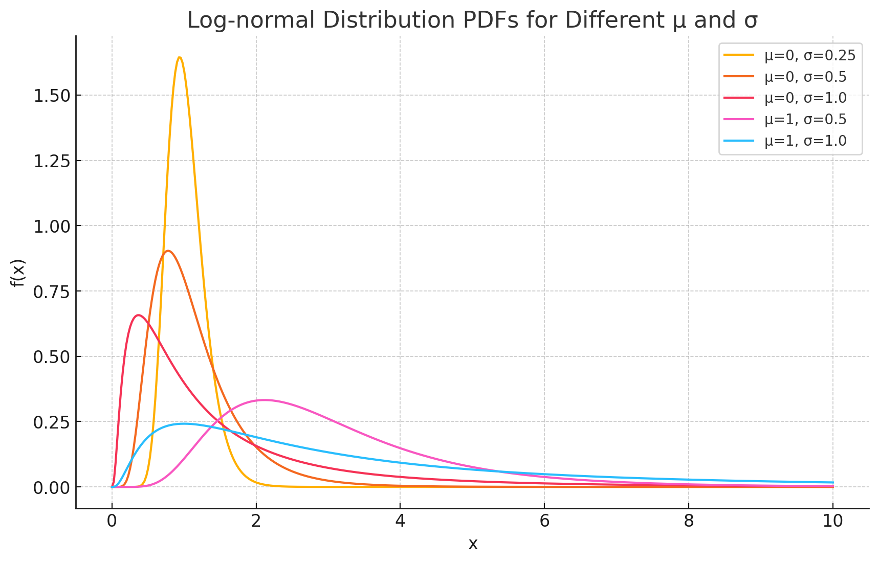
The Probability Density Function (PDF) of the log-normal distribution calculates the relative likelihood of a random variable taking on a specific value $x$.

The formula is:

\[f(x) = \frac{1}{x\sigma\sqrt{2\pi}} e^{-\frac{(\ln x - \mu)^2}{2\sigma^2}}\]

Where:

• $x$ is the random variable ($x > 0$).
• $\mu$ (mu) is the mean of the variable’s natural logarithm.
• $\sigma$ (sigma) is the standard deviation of the variable’s natural logarithm.
• $\ln x$ is the natural logarithm of $x$.

Intuition Behind the Formula

The formula allows us to understand the transformation from Normal to Log-Normal:

1. $(\ln x - \mu)^2$: This term reveals the core relationship. We are not measuring the distance of $x$ from the mean, but rather the distance of $\ln x$ from $\mu$. This confirms that the logarithm of the data follows a normal distribution.
2. $\frac{1}{x}$: This term (part of the scaling factor) is the Jacobian of the transformation. Because the logarithm compresses large numbers and expands small numbers between 0 and 1, this term is necessary to conserve probability mass, forcing the curve to be higher for small $x$ and lower for large $x$ (creating the skew).
3. $x > 0$ Constraint: The presence of $\ln x$ mathematically enforces that $x$ must be positive, as the logarithm of a negative number or zero is undefined.

Important Note: The Connection to Normal

The defining characteristic of a Log-Normal distribution is its relationship to the Normal distribution.

If a random variable $Y$ follows a Normal distribution:

\[Y \sim N(\mu, \sigma^2)\]

Then the variable $X$, defined as the exponential of $Y$, follows a Log-Normal distribution:

\[X = e^Y \sim \text{LogNormal}(\mu, \sigma^2)\]

This relationship allows us to analyze skewed data by simply taking the log of the data points and applying standard normal statistical methods.

Derivations

Deriving the properties of the Log-Normal distribution relies on using the substitution method to transform the integral back into the form of a Normal distribution.

Derivation of the Mean (E[X])

1. The Definition:

   \[E[X] = \int_{0}^{\infty} x \frac{1}{x\sigma\sqrt{2\pi}} e^{-\frac{(\ln x - \mu)^2}{2\sigma^2}} dx\]

   The $x$ in the numerator and the $x$ in the denominator cancel out.

2. Substitution: Let $y = \ln x$. Then $x = e^y$ and $dx = x dy = e^y dy$. However, since we already canceled the $x$’s, we essentially look at the expectation of $e^y$ where $y$ is Normal.

   \[E[X] = E[e^Y] \quad \text{where } Y \sim N(\mu, \sigma^2)\]

3. Using Moment Generating Functions: The expectation $E[e^Y]$ is the Moment Generating Function (MGF) of a Normal distribution evaluated at $t=1$. The MGF of a Normal distribution is $M_Y(t) = e^{\mu t + \frac{1}{2}\sigma^2 t^2}$.

4. Final Result: Set $t=1$:

   \[E[X] = e^{\mu + \frac{\sigma^2}{2}}\]

Derivation of the Variance (Var(X))

1. The Formula: We use $Var(X) = E[X^2] - (E[X])^2$. First, we need $E[X^2]$.

   \[E[X^2] = E[(e^Y)^2] = E[e^{2Y}]\]

2. Using MGF again: This is the MGF of the Normal distribution evaluated at $t=2$.

   \[E[X^2] = e^{\mu(2) + \frac{1}{2}\sigma^2(2)^2} = e^{2\mu + 2\sigma^2}\]

3. Calculate Variance:

   \[Var(X) = e^{2\mu + 2\sigma^2} - \left( e^{\mu + \frac{\sigma^2}{2}} \right)^2\] \[Var(X) = e^{2\mu + 2\sigma^2} - e^{2\mu + \sigma^2}\]

4. Final Result: Factor out the common term $e^{2\mu + \sigma^2}$:

   \[Var(X) = (e^{\sigma^2} - 1) e^{2\mu + \sigma^2}\]

Practical Examples

1. Financial Assets Scenario: An analyst is modeling the future price of a stock. Use Case: Stock prices cannot be negative, and price changes tend to compound over time (a 10% gain followed by a 10% gain is multiplicative). Therefore, the Log-Normal distribution is the standard model for asset prices in the Black-Scholes option pricing model.

2. Latent Periods of Diseases Scenario: An epidemiologist is studying the incubation period of a virus (time from infection to symptoms). Use Case: Most people might show symptoms within a few days (the peak), but a small number of people might take weeks to show symptoms (the long tail). The Log-Normal distribution accurately captures this “fast onset, slow tail” behavior.

3. Internet Traffic and Usage Scenario: A data scientist is analyzing the length of time users spend on a website or the file sizes of uploads. Use Case: The vast majority of sessions are short (seconds or minutes), but a few power users stay on for hours. Similarly, most files are small, but a few are massive. These metrics typically follow a Log-Normal distribution, and recognizing this prevents the mean from being skewed by the “whales” (extreme outliers).