Probability Distribution: Negative Binomial

The negative binomial distribution has two primary intuitions:

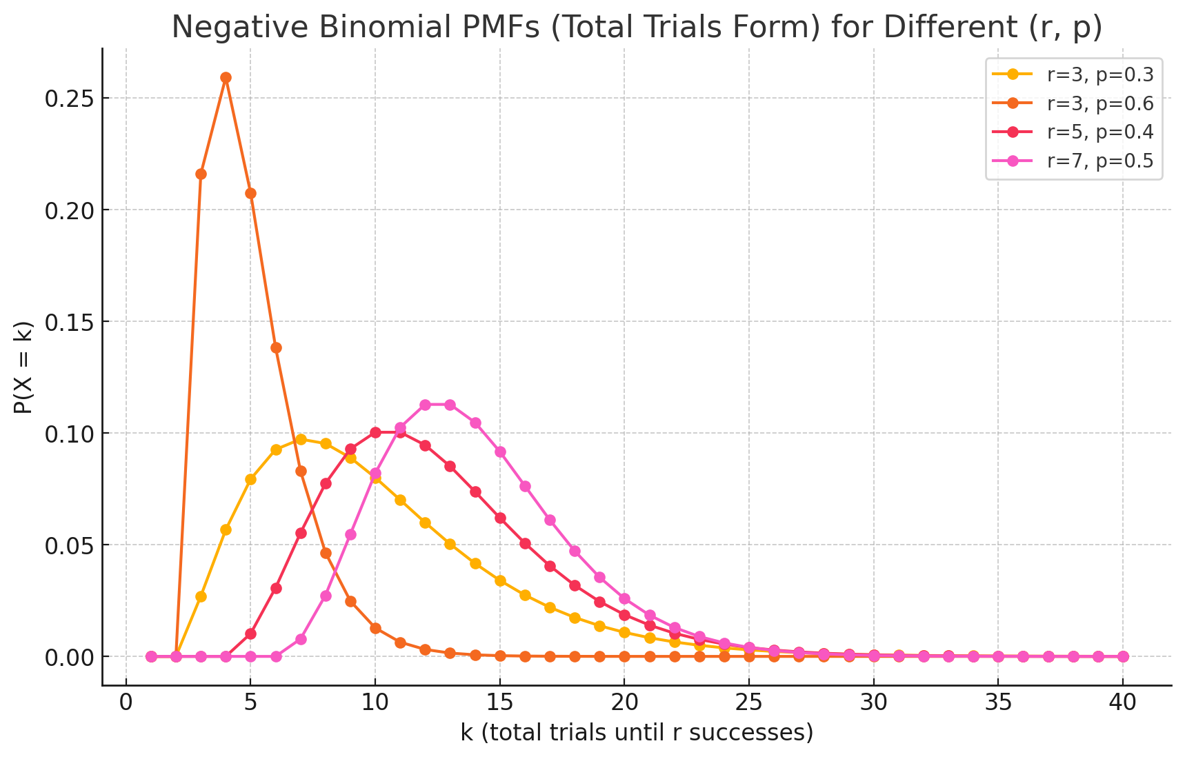
1. The “Waiting Time” Distribution: It models the number of trials ($k$) required to achieve a fixed number of successes ($r$). This is the opposite of the Binomial distribution, where you have a fixed number of trials and count the successes.
2. The “Overdispersed Count” Distribution: It models count data, like the Poisson distribution, but is more flexible because it can handle data where the variance is greater than the mean (a situation called overdispersion). This makes it ideal for real-world scenarios where events are not perfectly independent.

Probability Mass Function (PMF)

The Probability Mass Function (PMF) of the negative binomial distribution calculates the probability of needing exactly $k$ trials to achieve a predetermined $r$ number of successes.

The formula is:

\[P(X=k) = \binom{k-1}{r-1} p^r (1-p)^{k-r}\]

Where:

• k is the total number of trials (k = r, r+1, r+2, …).
• r is the fixed number of successes you want to achieve.
• p is the probability of success on any individual trial.
• $\binom{k-1}{r-1}$ is the binomial coefficient, which calculates the number of ways to arrange the first $r-1$ successes within the first $k-1$ trials.

Intuition Behind the Formula

The formula can be broken into three logical parts:

1. $p^r$: This is the probability of achieving your $r$ successes.
2. $(1-p)^{k-r}$: This is the probability of getting the $k-r$ failures that occur along the way.
3. $\binom{k-1}{r-1}$: This counts the number of different sequences in which the events can occur. The last event must be the $r$-th success, so we are calculating how many ways the first $r-1$ successes can be distributed among the previous $k-1$ trials.

Important Note: Alternative Formulation

Some textbooks and statistical software define the negative binomial distribution slightly differently: they model the number of failures ($y$) that occur before the $r$-th success is achieved.

In this version, the PMF is:

\[P(Y=y) = \binom{y+r-1}{r-1} p^r (1-p)^y\]

Where $y$ is the number of failures ($y$ = 0, 1, 2, …). This is the version used by libraries like SciPy in Python.

Derivations

The easiest way to derive the mean and variance is to think of a negative binomial random variable $X$ as the sum of $r$ independent and identical geometric random variables. Each geometric variable represents the number of trials needed for one success.

Derivation of the Mean (E[X])

1. The Model: Let $X = X_1 + X_2 + … + X_r$, where each $X_i$ is an independent geometric variable representing the trials needed for the i-th success.

2. Linearity of Expectation: The expected value of a sum is the sum of the expected values.

   \[E[X] = E[X_1] + E[X_2] + ... + E[X_r]\]
3. Mean of a Geometric Distribution: The mean of a single geometric distribution is $\frac{1}{p}$.

4. Final Result:

   \[E[X] = r \cdot \left(\frac{1}{p}\right) = \frac{r}{p}\]

Derivation of the Variance (Var(X))

1. The Model: We use the same model, $X = X_1 + X_2 + … + X_r$.

2. Variance of a Sum of Independents: Since the r geometric trials are independent, the variance of their sum is the sum of their variances.

   \[Var(X) = Var(X_1) + Var(X_2) + ... + Var(X_r)\]
3. Variance of a Geometric Distribution: The variance of a single geometric distribution is $\frac{1-p}{p^2}$.

4. Final Result:

   \[Var(X) = r \cdot \left(\frac{1-p}{p^2}\right) = \frac{r(1-p)}{p^2}\]

Practical Examples

1. Sales and Marketing Scenario: A marketing team wants to get 1,000 survey responses ($r=1000$). They know from experience that the probability of any given person responding is 5% ($p=0.05$). Use Case: The negative binomial distribution can calculate the probability that they will need to email exactly 21,000 people ($k=21000$) to reach their goal of 1,000 responses. It helps in planning the scale and cost of the campaign.

2. Manufacturing Quality Control Scenario: An inspector is checking light bulbs from a production line and needs to find 5 defective bulbs ($r=5$) to trigger a full line review. The known defect rate is 2% ($p=0.02$). Use Case: The distribution can model the number of bulbs the inspector will have to check before finding the fifth defective one. This helps in understanding the time and effort involved in quality control sampling.

3. Ecology and Epidemiology Scenario: An ecologist is studying the number of a rare insect species per quadrant in a field. The average might be low, but the insects tend to cluster together. This means some quadrants will have zero, and others will have many, leading to a variance much higher than the mean (overdispersion). Use Case: A Poisson distribution would be a poor fit here. The negative binomial distribution is the standard model in ecology for this type of clustered or “contagious” count data, as its extra parameter accurately captures the high variability.