Probability Distribution: Geometric

Probability Mass Function (PMF)

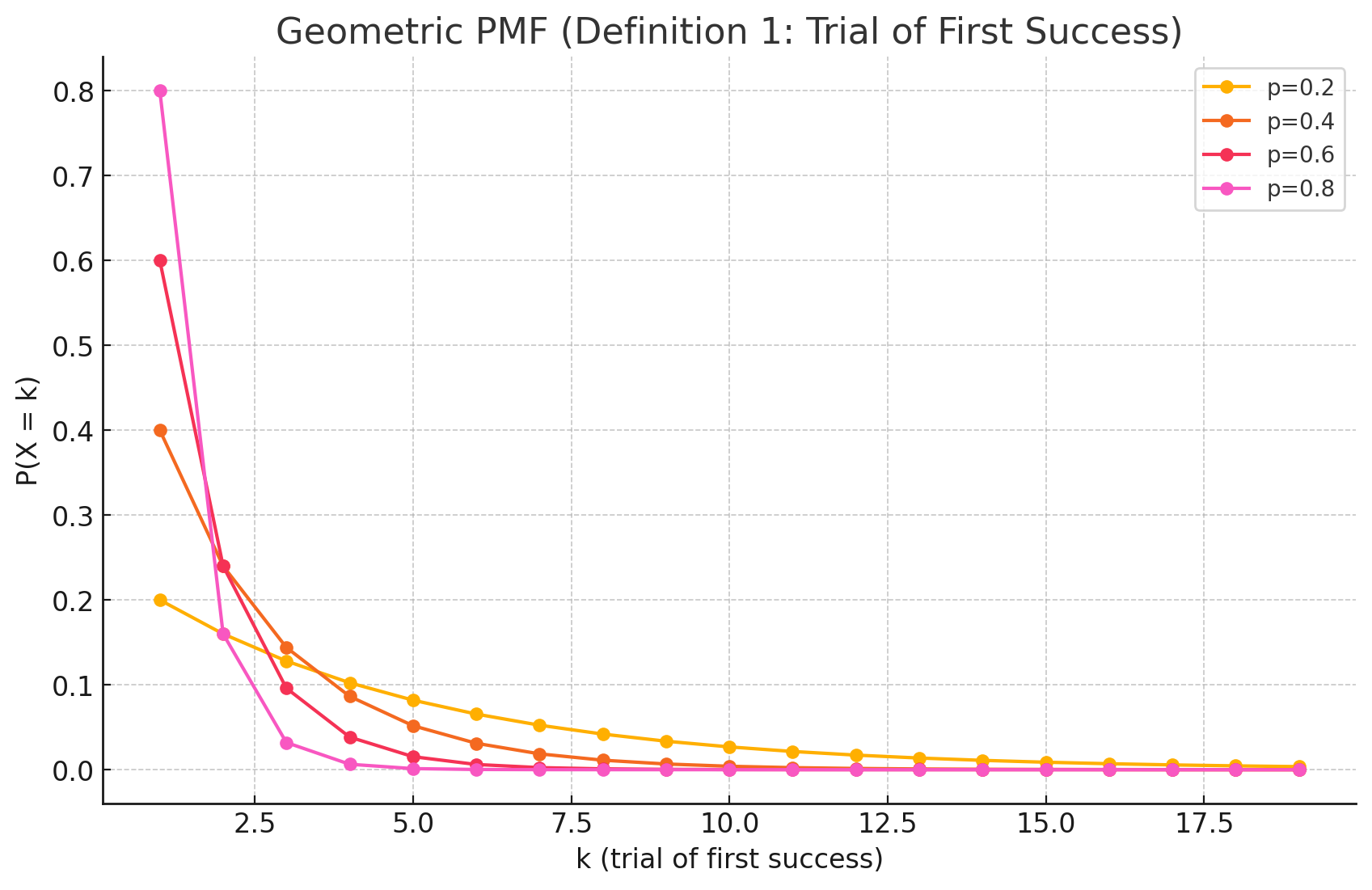
The Probability Mass Function (PMF) of the geometric distribution calculates the probability that the first success occurs exactly on the k-th trial.

The Formula

\[P(X=k) = (1-p)^{k-1} p\]

Where:

• k is the trial number of the first success ($k = 1, 2, 3, \dots$).
• p is the probability of success on any single trial.
• $(1-p)$ is the probability of failure (often denoted as $q$).

Intuition Behind the Formula

The logic is very straightforward if you think of the sequence of events required for the first success to happen specifically on trial $k$:

1. The Failures: You must fail every single time before the k-th trial. That means you need $k-1$ consecutive failures. The probability of this is $(1-p)^{k-1}$.
2. The Success: On the very next trial (the k-th one), you must succeed. The probability of this is $p$.
3. Combine them: Since the trials are independent, you multiply the probabilities together.

\[P(X=k) = \underbrace{(1-p) \times \dots \times (1-p)}_{\text{k-1 failures}} \times \underbrace{p}_{\text{1 success}}\]

Two Common Definitions

Note: In statistics, there are two slightly different ways to define “Geometric Distribution.”

1. Trials until success (The one defined above): Counts total attempts ($k=1, 2, 3…$). This is the most common definition in introductory statistics.
2. Failures before first success: Counts only the failures ($k=0, 1, 2…$). The formula for this version is $P(Y=k) = (1-p)^k p$.

Always check which definition is being used, specifically if you are using software libraries (e.g., Python’s scipy.stats.geom uses the first definition, starting at $k=1$).

Derivation of the Mean (E[X])

Derivations

Here are the derivations for the mean and variance of the geometric distribution. We’ll use $p$ for the probability of success and $q = 1-p$ for the probability of failure.

Derivation of the Mean (E[X])

The mean, or expected value $E[X]$, is the sum of all possible values of $k$ multiplied by their respective probabilities, $P(X=k) = q^{k-1}p$.

1. Definition of Expected Value:

   \[E[X] = \sum_{k=1}^{\infty} k \cdot P(X=k) = \sum_{k=1}^{\infty} k \cdot q^{k-1}p\]

2. Factor out p:

   \[E[X] = p \sum_{k=1}^{\infty} k \cdot q^{k-1}\]

3. Recognize the Derivative of a Geometric Series: The sum inside is a known power series. Recall the formula for an infinite geometric series:

   \[\sum_{k=0}^{\infty} q^k = \frac{1}{1-q}\]

   Differentiating both sides with respect to $q$ gives:

   \[\frac{d}{dq} \sum_{k=0}^{\infty} q^k = \sum_{k=1}^{\infty} k \cdot q^{k-1} = \frac{1}{(1-q)^2}\]

4. Substitute the Result: Now substitute this result back into the equation for $E[X]$:

   \[E[X] = p \cdot \frac{1}{(1-q)^2}\]

5. Final Simplification: Since $1-q = p$, we get the final formula:

   \[E[X] = p \cdot \frac{1}{p^2} = \frac{1}{p}\]

Derivation of the Variance (Var(X))

The variance is calculated using the formula $Var(X) = E[X^2] - (E[X])^2$. The key step is to first find $E[X^2]$. We do this by calculating $E[X(X-1)]$ and using the relation $E[X^2] = E[X(X-1)] + E[X]$.

1. Find E[X(X-1)]: This term is the second factorial moment and is related to the second derivative of the geometric series.

   \[E[X(X-1)] = \sum_{k=1}^{\infty} k(k-1) \cdot q^{k-1}p = p \sum_{k=1}^{\infty} k(k-1)q^{k-1}\]

   To find the sum, we differentiate the geometric series twice. We already have the first derivative:

   \[\sum_{k=1}^{\infty} k q^{k-1} = \frac{1}{(1-q)^2}\]

   Differentiating again with respect to $q$:

   \[\sum_{k=2}^{\infty} k(k-1)q^{k-2} = \frac{2}{(1-q)^3}\]

   To match our sum, we multiply by $q$:

   \[q \sum_{k=2}^{\infty} k(k-1)q^{k-2} = \sum_{k=2}^{\infty} k(k-1)q^{k-1} = \frac{2q}{(1-q)^3}\]

   Now substitute this back:

   \[E[X(X-1)] = p \cdot \frac{2q}{(1-q)^3} = p \cdot \frac{2q}{p^3} = \frac{2q}{p^2}\]

2. Calculate E[X²]:

   \[E[X^2] = E[X(X-1)] + E[X] = \frac{2q}{p^2} + \frac{1}{p} = \frac{2q+p}{p^2}\]

3. Calculate the Variance: Now we can plug everything into the variance formula:

   \[Var(X) = E[X^2] - (E[X])^2 = \frac{2q+p}{p^2} - \left(\frac{1}{p}\right)^2\] \[Var(X) = \frac{2q+p}{p^2} - \frac{1}{p^2} = \frac{2q+p-1}{p^2}\]

4. Final Simplification: Since $p+q=1$, we can say $p-1 = -q$.

   \[Var(X) = \frac{2q-q}{p^2} = \frac{q}{p^2}\]

   Substituting $q=1-p$ gives the final form:

   \[Var(X) = \frac{1-p}{p^2}\]

Practical Scenarios

Scenario 1: Quality Control - Destructive Testing

Situation: A car manufacturer performs destructive crash tests on a new bumper design. The probability of the bumper failing a specific stress test is 5% ($p = 0.05$). The engineers want to know the probability that they will have to test exactly 10 bumpers before observing the first failure.

Derivation: We use the Geometric PMF with $p = 0.05$ and $k = 10$.

\[P(X=10) = (1 - 0.05)^{10-1} \times 0.05\] \[P(X=10) = (0.95)^9 \times 0.05\] \[P(X=10) \approx 0.6302 \times 0.05 \approx 0.0315\]

There is approximately a 3.15% chance that the first failure will occur precisely on the 10th test. This helps in budgeting for the number of test units required.

Scenario 2: Sales Prospecting

Situation: A software salesperson makes cold calls to potential clients. Historically, they have a 10% success rate ($p = 0.10$) of booking a meeting from a cold call. They want to calculate the likelihood that they will make their first successful booking on their 5th call of the day.

Derivation: We use the Geometric PMF with $p = 0.10$ and $k = 5$.

\[P(X=5) = (1 - 0.10)^{5-1} \times 0.10\] \[P(X=5) = (0.90)^4 \times 0.10\] \[P(X=5) = 0.6561 \times 0.10 \approx 0.0656\]

There is roughly a 6.6% chance that the salesperson’s first success will happen on exactly the 5th call. This type of modeling helps managers set realistic activity targets for sales teams.