Probability Distribution: Normal (Gaussian)

The Normal (or Gaussian) distribution has two primary intuitions:

1. The “Bell Curve” of Nature: It models natural phenomena where most observations cluster around a central mean, with extreme values becoming increasingly rare as you move away from the center. It implies symmetry and predictability.
2. The “Sum of Many Parts” Distribution: Based on the Central Limit Theorem, it describes the distribution of the sum (or average) of many independent random variables. This is why it appears everywhere, from biological heights to measurement errors, even if the underlying source data isn’t normal.

Probability Density Function (PDF)

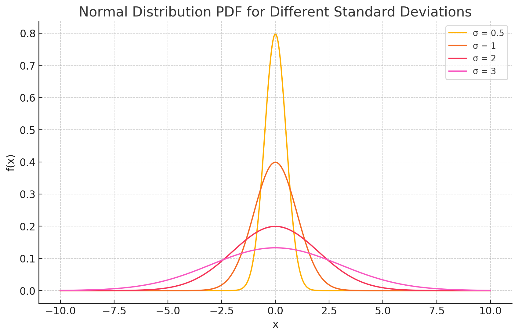
The Probability Density Function (PDF) of the normal distribution calculates the relative likelihood of a random variable taking on a specific value $x$. Unlike the PMF for discrete distributions, probabilities here are calculated as the area under the curve.

The formula is:

\[f(x) = \frac{1}{\sigma\sqrt{2\pi}} e^{-\frac{1}{2}\left(\frac{x-\mu}{\sigma}\right)^2}\]

Where:

• $x$ is the value of the random variable ($-\infty < x < \infty$).
• $\mu$ (mu) is the mean or center of the distribution.
• $\sigma$ (sigma) is the standard deviation, measuring the spread.
• $\sigma^2$ is the variance.

Intuition Behind the Formula

The formula can be broken into three logical parts:

1. $(x-\mu)^2$: This term measures the distance from the mean. Squaring it ensures that deviations to the left (negative) and right (positive) are treated equally, creating symmetry.
2. $e^{-\frac{1}{2}(\dots)}$: The exponential decay ensures that as $x$ gets further from $\mu$, the probability density drops rapidly toward zero. This creates the “bell” shape with tails.
3. $\frac{1}{\sigma\sqrt{2\pi}}$: This is a scaling factor (normalization constant). It ensures that the total area under the curve equals exactly 1, which is a requirement for any valid probability distribution.

Important Note: The Standard Normal

A specific case of this distribution is the Standard Normal Distribution, where $\mu = 0$ and $\sigma = 1$. This is often used to compare different datasets by converting values into Z-scores.

The PDF simplifies to:

\[\phi(z) = \frac{1}{\sqrt{2\pi}} e^{-\frac{z^2}{2}}\]

This standardization allows for the use of Z-tables to find probabilities regardless of the original units of measurement.

Derivations

Deriving the mean and variance involves calculus, specifically integrating the PDF over the entire range of real numbers.

Derivation of the Mean (E[X])

1. The Definition: The expected value is the integral of $x$ times the density function.

   \[E[X] = \int_{-\infty}^{\infty} x \frac{1}{\sigma\sqrt{2\pi}} e^{-\frac{(x-\mu)^2}{2\sigma^2}} dx\]

2. Substitution: Let $z = \frac{x-\mu}{\sigma}$. Then $x = \sigma z + \mu$ and $dx = \sigma dz$.

   \[E[X] = \int_{-\infty}^{\infty} (\sigma z + \mu) \frac{1}{\sqrt{2\pi}} e^{-\frac{z^2}{2}} dz\]
3. Splitting the Integral: The term with $z e^{-z^2/2}$ is an odd function centered at 0, so its integral over the symmetric range is 0. The remaining term is $\mu$ times the integral of the standard normal PDF (which is 1).

4. Final Result:

   \[E[X] = 0 + \mu(1) = \mu\]

Derivation of the Variance (Var(X))

1. The Definition: Variance is defined as $E[(X-\mu)^2]$.

   \[Var(X) = \int_{-\infty}^{\infty} (x-\mu)^2 \frac{1}{\sigma\sqrt{2\pi}} e^{-\frac{(x-\mu)^2}{2\sigma^2}} dx\]

2. Substitution: Using the same substitution $z = \frac{x-\mu}{\sigma}$, we get $(x-\mu)^2 = \sigma^2 z^2$.

   \[Var(X) = \frac{\sigma^2}{\sqrt{2\pi}} \int_{-\infty}^{\infty} z^2 e^{-\frac{z^2}{2}} dz\]
3. Integration by Parts: We solve the integral using integration by parts, where $u=z$ and $dv = z e^{-z^2/2} dz$. The result of the integral part is $\sqrt{2\pi}$.

4. Final Result:

   \[Var(X) = \frac{\sigma^2}{\sqrt{2\pi}} (\sqrt{2\pi}) = \sigma^2\]

Practical Examples

1. Biological Measurements Scenario: An anthropologist is studying the height of adult males in a specific region. Use Case: Human heights typically follow a normal distribution. By calculating the mean ($\mu$) and standard deviation ($\sigma$) of a sample, the anthropologist can determine the probability that a randomly selected individual is above a certain height (e.g., probability of being taller than 6 feet) or identify outliers (e.g., gigantism).

2. Standardized Testing Scenario: An education board administers a standardized test like the SAT or GRE. The scores are designed to be normally distributed with a mean of 1000 and a standard deviation of 200. Use Case: The board uses the distribution to assign percentiles. If a student scores 1400, the board calculates their Z-score ($Z=2$) and determines they performed better than roughly 97.7% of the population.

3. Financial Risk Management Scenario: An investment firm models the daily returns of a “blue chip” stock portfolio. While not perfectly normal (due to “fat tails”), returns are often approximated as normal for basic risk assessment. Use Case: Using the normal distribution, analysts calculate Value at Risk (VaR). They might determine that there is a 5% chance ($\approx 1.65$ standard deviations below the mean) that the portfolio will lose more than $10,000 in a single day.