Probability Distribution: Laplace

The Laplace distribution (often called the “Double Exponential” distribution) has two primary intuitions:

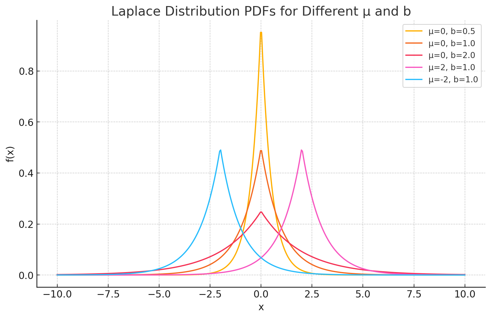
1. The “Peakier” Bell Curve: Visually, it looks like two exponential distributions spliced together back-to-back. Compared to the Normal distribution, it has a sharper peak at the mean and fatter tails. This makes it a better model for data that is concentrated around a central value but has more frequent extreme outliers than a Gaussian model predicts.
2. The “Difference of Two Exponentials” Distribution: Mathematically, if you take two independent random variables that follow an exponential distribution and subtract one from the other, the result follows a Laplace distribution. This intuition is key in fields like signal processing and finance.

Probability Density Function (PDF)

The Probability Density Function (PDF) of the Laplace distribution calculates the relative likelihood of a random variable taking on a specific value $x$.

The formula is:

\[f(x) = \frac{1}{2b} e^{-\frac{|x-\mu|}{b}}\]

Where:

• $x$ is the value of the random variable ($-\infty < x < \infty$).
• $\mu$ (mu) is the location parameter (mean/median/mode).
• $b$ (b) is the scale parameter ($b > 0$), which determines the spread.
• The variance is $2b^2$.

Intuition Behind the Formula

The formula can be broken into three logical parts:

1. $\lvert x-\mu \rvert$: This term measures the absolute distance from the location parameter. Unlike the Normal distribution which uses the squared distance $(x-\mu)^2$, the Laplace uses the absolute difference. This is what creates the sharp “tent-like” peak at the center rather than a smooth bell curve.
2. $e^{-\frac{\lvert \dots \rvert}{b}}$: The exponential decay ensures that probability drops as you move away from $\mu$. The rate of this decay is controlled by $b$.
3. $\frac{1}{2b}$: This is the normalization constant. It ensures that the total area under the curve equals exactly 1.

Important Note: Connection to Median

While the Normal distribution is associated with the mean (minimizing squared error), the Laplace distribution is deeply connected to the median. In regression analysis, minimizing the absolute error (L1 regularization or Lasso) implies an assumption that the errors follow a Laplace distribution.

Derivations

Deriving the mean and variance involves integrating the PDF. The presence of the absolute value function requires splitting the integral into two parts: one from $-\infty$ to $\mu$ and one from $\mu$ to $\infty$.

Derivation of the Mean (E[X])

1. The Definition:

   \[E[X] = \int_{-\infty}^{\infty} x \frac{1}{2b} e^{-\frac{\lvert x-\mu \rvert}{b}} dx\]
2. Splitting the Integral: We split the range at $\mu$.
   • For $x < \mu$, $\lvert x-\mu \rvert = -(x-\mu)$.
   • For $x > \mu$, $\lvert x-\mu \rvert = (x-\mu)$.

   This creates two integrals involving exponential terms. However, due to the symmetry of the distribution around $\mu$, the terms involving deviations from the mean cancel out perfectly.

3. Symmetry Argument: The function $x \cdot f(x)$ is symmetric around $\mu$. Just like the Normal distribution, the “pull” from the left tail exactly balances the “pull” from the right tail.

4. Final Result:

   \[E[X] = \mu\]

Derivation of the Variance (Var(X))

1. The Definition: Variance is defined as $E[(X-\mu)^2]$.

   \[Var(X) = \int_{-\infty}^{\infty} (x-\mu)^2 \frac{1}{2b} e^{-\frac{\lvert x-\mu \rvert}{b}} dx\]

2. Shift and Symmetry: Let $y = x - \mu$. The integral becomes centered at 0. Because $(y)^2$ and the PDF are symmetric, we can integrate from 0 to $\infty$ and multiply by 2.

   \[Var(X) = 2 \int_{0}^{\infty} y^2 \frac{1}{2b} e^{-\frac{y}{b}} dy = \frac{1}{b} \int_{0}^{\infty} y^2 e^{-\frac{y}{b}} dy\]
3. Gamma Function / Integration by Parts: This integral fits the form of the Gamma function $\Gamma(n) = \int x^{n-1}e^{-x}dx$, or can be solved via repeated integration by parts. The integral evaluates to $2b^3$.

4. Final Result:

   \[Var(X) = \frac{1}{b} (2b^3) = 2b^2\]

Practical Examples

1. Hydrology and Environmental Events Scenario: A hydrologist is modeling extreme river flow events or flood peaks over a long period. Use Case: While average water levels might be normal, extreme flood events often have “fatter tails” than a normal distribution predicts. The Laplace distribution is often used to model these sharper peaks and heavier tails to better estimate the risk of catastrophic floods.

2. Speech Recognition Scenario: An engineer is processing speech signals. They look at the distribution of the signal amplitudes (specifically the DFT coefficients) over a short time window. Use Case: In speech, there are many small values (silence or background noise) and fewer large values (strong vocal peaks). The Laplace distribution fits this data much better than a Normal distribution because of its sharp peak at zero and heavy tails, allowing for more effective compression and noise reduction algorithms.

3. Machine Learning (Regularization) Scenario: A data scientist is building a regression model with thousands of features and wants to perform feature selection. Use Case: The scientist uses Lasso Regression (L1 regularization). This technique adds a penalty term equivalent to assuming the coefficients follow a Laplace distribution (centered at zero). Because of the Laplace distribution’s sharp peak at zero, the model drives many coefficients to exactly zero, effectively selecting only the most important features.