Training LLMs on a Budget: LoRA, QLoRA, and LoftQ
- LLM sampling techniques
- Temperature
- KV cache
- Prompt caching
- RAG evaluation
- Linear quantization
- Non-linear quantization
- AWQ
- GPTQ
- LoRA, QLoRA, and LoftQ You are here
So far in this series, quantization has been a serving story - shrink a trained model so it fits on cheaper hardware and runs faster. In the linear quantization article we set up the uniform grid and affine formulas. In the non-linear article we reshaped the grid to fit bell-curved weights, and NF4 emerged as the practical sweet spot.
But NF4 has a second act that is arguably more consequential than anything it does on the inference side. That second act is on the training side - specifically, making it possible to fine-tune enormous pre-trained models on a single consumer GPU.
To see why this matters, let’s look at the cost of fine-tuning a 70B model in full precision. Weights alone are 140 GB in FP16. Add gradients (another 140 GB) and the Adam optimizer’s two state tensors in FP32 (about 560 GB), and we’re looking at roughly 840 GB just to hold the training state, before we even load a single token of data. That’s a small datacentre. The question this article answers is: can we bring that bill down to something a 24 GB consumer card can handle?
The answer is yes, in three steps that build on each other:
- LoRA - freeze the base model and train a tiny, low-rank adapter on top. Collapses the optimizer bill to near zero.
- QLoRA - also quantize the frozen base to NF4 so the weights themselves fit in memory.
- LoftQ - initialize the adapter so the quantized base starts training already correct, instead of spending early steps undoing quantization error.
Each step tightens the budget further, and each reveals something worth understanding. Let’s walk through them.
1. The memory bill of fine-tuning
Before any tricks, let’s be concrete about where the memory actually goes. For each trainable parameter in a BF16 mixed-precision setup with the Adam optimizer, the accounting used in the QLoRA paper and the de facto default for LLM fine-tuning on A100/H100-class hardware is shown below:
| Tensor | Dtype | Bytes / param |
|---|---|---|
| Weights | BF16 | 2 |
| Gradients | BF16 | 2 |
| Adam first moment $m$ | FP32 | 4 |
| Adam second moment $v$ | FP32 | 4 |
| Total | 12 |
That’s the headline number: 12 bytes per parameter for full fine-tuning in this configuration. It is a common accounting, not an unavoidable floor: the count shifts with the optimizer (SGD-momentum keeps one moment, not two; 8-bit optimizers halve the state), with whether the framework keeps FP32 master weights (see below), and with sharding strategy (ZeRO/FSDP spread these tensors across GPUs). And it covers only the persistent training state - activation memory, attention/KV intermediates, temporary workspaces, and allocator fragmentation all stack on top, and can dominate at long sequence lengths. Treat 12 bytes/param as a persistent-state estimate to reason with, then measure peak VRAM for the real number. (Units: GB = $10^9$ bytes; a “24 GB” card is ~22.4 GiB addressable, so leave headroom.)
A caveat about the FP32 master copy of the weights that many mixed-precision recipes keep. It exists for precision retention, not a headline underflow: a single optimizer update, learning_rate × gradient, is often far smaller than the weight it modifies, and added directly to a low-precision weight it can round away to nothing (the weight’s representable step is larger than the update), so it is silently lost step after step. Keeping the weights in FP32 for the addition preserves those accumulations, at +4 bytes/param - 16 bytes per parameter when a master copy is used. BF16’s wider exponent range eases the pressure (hence the 12-byte no-master shorthand) but does not make a master copy universally unnecessary; many BF16 recipes still keep one or use stochastic rounding. This article uses 12 bytes; scale by 16/12 for a master-copy setup (~1,120 GB for a 70B model).
| Model | Full-FT memory (no activations) |
|---|---|
| 7B | 84 GB |
| 13B | 156 GB |
| 65B | 780 GB |
| 70B | 840 GB |
A single 24 GB RTX 4090 can’t even hold the weights of a 13B model at this setting, let alone train them. An 80 GB H100 can train a 7B model with some care, and needs a multi-GPU cluster for anything bigger.
The leverage point is where the memory actually lives. Of the 12 bytes per parameter, 10 of them are gradients and optimizer states, and those are only needed for parameters we actually train. If we could make 99.9 % of the parameters untrainable, we’d immediately drop those 10 bytes from 99.9 % of the model. That is exactly LoRA’s move.
2. LoRA - the low-rank adapter trick
The intuition
Here’s the empirical observation behind LoRA (Hu et al., 2021): the update $\Delta W$ that fine-tuning applies to a pre-trained weight matrix is approximately low-rank. Adapting a generalist language model to something like legal document summarisation doesn’t require moving every direction in weight space, a handful of task-relevant directions is enough. The pre-training did the hard work of learning features. Fine-tuning just picks out the few that matter for the new task and reweights them.
If that update is genuinely low-rank, we can parameterize it as a product of two tiny matrices instead of one big one, and only train those.
To see what “approximately low-rank” actually looks like, here’s the singular value spectrum of a synthetic $\Delta W$ built to mimic a real fine-tuning delta - a small rank-8 task signal on top of a lot of low-magnitude noise across all other directions:
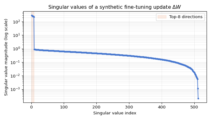
The top 8 singular values sit 2–3 orders of magnitude above the rest. That gap is the reason LoRA’s rank-$r$ parametrisation captures most of the useful update while ignoring almost the entire matrix.
The math
Freeze the pre-trained weight matrix $W \in \mathbb{R}^{d_{out} \times d_{in}}$. Introduce two new matrices
\[A \in \mathbb{R}^{r \times d_{in}}, \qquad B \in \mathbb{R}^{d_{out} \times r}, \qquad r \ll \min(d_{in}, d_{out})\]and define the effective forward pass as:
\[y = Wx + \frac{\alpha}{r} BAx\]The original matrix never moves. Only $A$ and $B$ are trainable, and their product $BA$ has rank at most $r$ - exactly the low-rank update we wanted.
The extra factor $\alpha/r$ is the LoRA scaling, not optional decoration. $\alpha$ is a fixed hyperparameter (often $\alpha = r$ or $2r$); dividing by $r$ keeps the update’s magnitude roughly constant as we sweep the rank, so the learning rate need not be re-tuned each time (rank-stabilized LoRA divides by $\sqrt{r}$ instead). The scaling is part of the layer, so it reappears wherever $BA$ does - the merge step and LoftQ’s init both carry it.
Initialization matters
A subtle but critical detail: $A$ is initialised to a small random Gaussian, $B$ is initialized to zero. That way $BA = 0$ at step 0, and the forward pass is bit-identical to the frozen base model. Training starts from the pre-trained output, not some random perturbation of it.
Why this specific assignment - random $A$, zero $B$ - rather than the reverse? The forward pass at step 0 is identical either way (both give $BA = 0$), so it isn’t about the initial output. The difference shows up in the first gradient step, and to see it we need the chain rule.
A word on the loss $L$ first. For an LLM, $L$ is almost always cross-entropy over the next-token prediction, averaged across the batch (for a regression-style head it might be MSE instead). For this argument, though, we don’t actually need to pick one. The only thing the derivation relies on is that $L$ is some differentiable scalar function of the output vector $y$, so that the upstream gradient $\partial L / \partial y$ is a well-defined vector of the same shape as $y$. Whatever $L$ turns out to be in practice, the logic below is agnostic.
Why introduce an intermediate $z = Ax$? The LoRA contribution $BAx$ is a composition of two linear maps: first $x \mapsto Ax$, then that result gets multiplied by $B$. The chain rule is cleanest when we take one map at a time, so it helps to give the in-between quantity a name:
\[z = Ax \quad (\text{shape } r \times 1)\]The forward pass becomes $y = Wx + Bz$. Now $A$ sits in the first linear map and $B$ in the second, and we can differentiate through each link in turn.
First link: gradient from $y$ back to $z$. Before we write anything down, a note on indices. We’ll use $i$ for the output index - it ranges over the $d_{out}$ components of $y$ (and picks out which row of $B$ we’re looking at). We’ll use $k$ for the intermediate index - it ranges over the $r$ components of $z$ (and picks out which column of $B$ we’re looking at). So $B_{ik}$ means “row $i$, column $k$ of $B$”, the entry that multiplies the $k$-th component of $z$ when producing the $i$-th component of $y$.
The output depends on $z$ only through the $Bz$ term, so writing it component-wise, \(y_i = (Wx)_i + \sum_k B_{ik} z_k\), which gives $\partial y_i / \partial z_k = B_{ik}$. The chain rule then gives:
\[\frac{\partial L}{\partial z_k} \;=\; \sum_i \frac{\partial L}{\partial y_i} \cdot \frac{\partial y_i}{\partial z_k} \;=\; \sum_i B_{ik} \cdot \frac{\partial L}{\partial y_i}\]The sum contracts over the output index $i$, the $z$-index $k$ ends up playing the role of the row. That index swap is exactly what turns into a transpose when we write the same thing in matrix form:
\[\frac{\partial L}{\partial z} \;=\; B^T \cdot \frac{\partial L}{\partial y}\](This is just the standard backprop rule for a linear layer, rederived. Mnemonic: the gradient flows backward through $y = Bz$ by multiplying by $B^T$ - the indices that are contracted on the forward pass are the ones that get contracted again on the backward pass, and preserving shapes forces the transpose.)
Second link: gradient from $z$ back to $A$. From $z = Ax$ the same reasoning gives $\partial L / \partial A = (\partial L / \partial z) \cdot x^T$. Chaining the two links together:
\[\frac{\partial L}{\partial A} \;=\; B^T \cdot \frac{\partial L}{\partial y} \cdot x^T\]That’s where the $B^T$ factor comes from - not a coincidence, but what the chain rule always leaves behind when the gradient has to flow back through $B$ before it can reach $A$. The derivation for $B$ is simpler because $B$ is the outermost linear map: $\partial L / \partial B = (\partial L / \partial y) \cdot z^T$, and substituting $z = Ax$ gives:
\[\frac{\partial L}{\partial B} \;=\; \frac{\partial L}{\partial y} \cdot x^T \cdot A^T\]Now look at step 0 under the two candidate initialisations:
| Init | $\partial L / \partial A$ at step 0 | $\partial L / \partial B$ at step 0 |
|---|---|---|
| $A$ random, $B = 0$ (convention) | 0 (killed by $B^T = 0$) | non-zero |
| $A = 0$, $B$ random (swapped) | non-zero | 0 (killed by $A^T = 0$) |
In both cases, one of the two matrices updates at step 0 and the other sits still. Once the first one becomes non-zero, the other starts updating on the next step. So both initialisations do train - neither is a hard failure.
The reason the community settled on random-$A$, zero-$B$ is about the scale of those first updates. When $A$ is random-Gaussian and $B = 0$, the first non-zero gradient is on $B$, and it’s proportional to $A^T$ - a product of a well-behaved task gradient and a well-scaled random matrix. When the roles are swapped, the first non-zero gradient lands on $A$ and is proportional to $B^T$ - a random matrix again, but one that was initialised without the careful variance scaling typically applied to weights like $A$. In practice the convention gives steadier early dynamics, especially once the LoRA scaling factor $\alpha/r$ is thrown in. It’s a convention, but a well-motivated one.
A worked parameter count
Take LLaMA-7B: hidden dimension 4096, 32 transformer layers. We’ll follow the original LoRA paper’s setup and adapt only the query and value projections ($q_{\text{proj}}$, $v_{\text{proj}}$) in each layer - each $4096 \times 4096$. That q/v-only choice is a historical default, not a rule: many current recipes adapt all attention projections ($q, k, v, o$) and the MLP matrices too. Target-module choice is an empirical capacity/memory trade; we use q/v here to keep the arithmetic clean.
With $r = 8$, each LoRA-adapted matrix adds:
\[|A| + |B| = r \cdot d_{in} + d_{out} \cdot r = 8 \cdot 4096 + 4096 \cdot 8 = 65{,}536 \text{ params}\]Across $2 \times 32 = 64$ adapted matrices, total trainable parameters come to about 4.2 million - roughly 0.06 % of the 7 B base.
The memory picture changes dramatically:
| Tensor | Full FT (7B) | LoRA (7B, $r=8$) |
|---|---|---|
| Base weights (frozen) | 14 GB | 14 GB |
| Gradients | 14 GB | 8 MB |
| Adam $m + v$ (FP32) | 56 GB | 34 MB |
| Total | 84 GB | ~14 GB |
The optimizer bill collapses from 56 GB to 34 MB, because optimizer state scales with trainable parameters, not total parameters. A 7B model becomes LoRA-fine-tunable on a single 24 GB card with plenty of headroom for activations.
Deployment: keep or merge
At inference time we have two choices. We can keep the adapters separate and compute $y = Wx + \frac{\alpha}{r}BAx$ - this costs one extra matmul per layer, but it lets us hot-swap adapters for different tasks. Or we can merge them once training is done:
\[W' \leftarrow W + \frac{\alpha}{r} BA\]and deploy $W’$ as a drop-in replacement for the original weight matrix, with no extra matmul at serving time. One caveat: clean merging assumes a full-precision base. When the base is quantized (as in QLoRA below), merging an FP16 adapter into it requires dequantizing, adding $\frac{\alpha}{r}BA$, and re-quantizing - which shifts the numerics slightly and gives up the ability to swap adapters. So “merge for zero overhead” is a property of the FP16-base case; on a quantized base it is a deliberate trade, not a free lunch.
What LoRA does not solve
LoRA shrinks the gradient and optimizer memory, but the frozen base $W$ still sits in GPU memory at FP16. For a 7B model that’s 14 GB - fine on a 24 GB card. For a 65B model that’s 130 GB - still out of reach for anything but a multi-GPU cluster. The base weights are the next thing to attack.
3. QLoRA - LoRA on a 4-bit quantized base
QLoRA (Dettmers et al., 2023) makes one delightfully simple observation: the base model is frozen during LoRA training. We never touch it. So why keep it in FP16 at all? If we quantize it to NF4, it shrinks by 4× - and the training loop barely notices.
QLoRA is not quantization-aware training (QAT). Worth stating plainly, since the two are easy to conflate. QAT optimizes the base weights themselves through a simulated low-precision path, so the model learns to be quantization-robust. QLoRA does the opposite: the quantized base is frozen; gradients flow through an on-the-fly dequantization only to reach the small BF16 adapters, which are what train. It is quantized parameter-efficient fine-tuning, not QAT - the §6 taxonomy table lines the two up.
The setup
Before training starts, quantize the base weights $W$ once to NF4 and store them that way for the rest of training. Keep the LoRA adapters $A, B$ in BF16 and train them normally. The forward pass becomes:
\[y = \text{dequant}_{\text{NF4}}(W_q) \cdot x \;+\; BA \cdot x\]At each forward pass, the NF4 base is dequantized block-by-block to BF16 on the fly, the matmul is computed, and the dequantized tensor is discarded. The stored form stays NF4, which is what keeps memory low.
Why this works at all
A fair question to pause on: won’t the quantization error in $W_q$ degrade training? Here’s the reassuring bit. Because the base is frozen, its quantization error $\epsilon = W - \text{dequant}(W_q)$ is a constant bias throughout training - it doesn’t shift between steps. And the LoRA adapters are trained by gradient descent on the loss that sits on top of the quantized base. So during training, $BA$ quietly ends up absorbing whatever part of $\epsilon$ turns out to be task-relevant, along with the task-specific update, all in one optimisation.
In other words: QLoRA doesn’t pretend the quantized base equals the original; it lets the adapters learn to compensate. Two qualifiers: the adapters can only absorb the part of $\epsilon$ in their rank-$r$ subspace (the rest is permanent), and “the adapters compensate” is an empirical tendency to measure against a same-recipe baseline, not a theorem. It holds well at 4-bit and frays as bits drop - which is what motivates LoftQ.
The three QLoRA tricks
1. NF4 for the base. This is the same NF4 from the non-linear quantization article - 16 quantile points drawn from the inverse CDF of a standard normal, applied block-wise to handle outliers. Recap in one sentence: LLM weights are bell-curved, so a grid with more bins near zero and fewer at the tails loses less precision than a uniform grid at the same bit-width. No new machinery here; we’re just reusing it.
2. Double quantization. NF4 uses block-wise absmax scaling - one FP32 scaling constant per block of 64 weights. That overhead is not free:
\[\text{scaling overhead} = \frac{32 \text{ bits}}{64 \text{ weights}} = 0.5 \text{ bits per weight}\]Half a bit per parameter sounds small, but at 65 B parameters it’s ~4 GB of pure overhead. QLoRA quantizes those scaling constants themselves - 8-bit FP8 with a second-level absmax over blocks of 256 first-level constants. The overhead drops to:
\[\underbrace{\frac{8 \text{ bits}}{64}}_{\text{first level (FP8)}} \;+\; \underbrace{\frac{32 \text{ bits}}{64 \times 256}}_{\text{second level (FP32)}} \;\approx\; 0.127 \text{ bits per weight}\]Net savings: about 0.373 bits per weight. Worth the trouble at scale.
3. Paged optimizers. Not a numerical trick - a memory-management safety valve. During gradient update spikes, NVIDIA unified memory transparently swaps optimizer state out to CPU RAM instead of OOMing. Conceptually it’s just swap space for training, surfaced through the CUDA driver. It is a resilience mechanism, not free memory: the CPU-GPU transfers can stall the step, so paging that fires every iteration signals a genuinely undersized GPU, not a solved problem.
The memory table
For a 65 B model, here’s how the base-weight memory shakes out across three configurations:
| Configuration | Bits/weight | Memory (65 B) |
|---|---|---|
| FP16 base | 16 | 130 GB |
| NF4 base (no DQ) | 4.5 | 36.6 GB |
| NF4 base + Double Quant | 4.127 | 33.5 GB |
Add LoRA adapter + optimizer on top of the NF4+DQ row - a few hundred MB for any reasonable rank - and the whole training state lands around 35 GB. That’s a 48 GB A6000. A 65B model, trainable on one card - precisely the QLoRA paper’s headline demonstration (65B on a single 48 GB GPU). Activations still stack on top, so treat 35 GB as the persistent-state figure.
What QLoRA leaves open
The base model’s quantization is decided once at the start of training and never revisited. The adapters learn to compensate within their rank-$r$ budget, but any part of the quantization error that doesn’t lie in their rank-$r$ subspace is permanent. At 4-bit this is usually fine. At 3-bit or 2-bit it becomes a problem - the quantization error is larger, and a naive init where $BA = 0$ means the effective weight matrix at step 0 is strictly worse than the original. Training has to spend time undoing quantization before it can learn the task.
This is the gap LoftQ closes.
4. LoftQ - initialising the adapter so the base starts (almost) correct
The problem in one picture
Let’s set the downstream task aside for a moment and look just at what the model sees. At step 0 of QLoRA training, the effective weight matrix is:
\[W_{\text{effective}}^{(0)} \;=\; W_q \;+\; B_0 A_0 \;=\; W_q\]because $B_0 = 0$ initialisation makes $BA$ vanish at the start. So the model begins training from a strictly degraded version of the original - worse than the pre-trained base by exactly the NF4 quantization error. The first thousand steps of training are partly spent using the adapter to claw back toward $W$, not to learn the downstream task. That wastes adapter capacity and, at low bit-widths, can prevent convergence entirely.
LoftQ (Li et al., 2023) asks: can we pick $A_0, B_0$ so that $W_q + B_0 A_0 \approx W$ from the very first step? The precise goal is narrower than “start correct”: LoftQ minimizes the initial weight-reconstruction error $\lVert W - (W_q + B_0 A_0) \rVert_F$, so training starts much closer to the original model rather than exactly at it. That is not the same as a guarantee about downstream task quality - a smaller init residual tends to help and is what unlocks the very-low-bit regime, but the actual task metric still has to be measured. What LoftQ removes is the wasted early training spent clawing back from quantization damage; how much that buys depends on the model, the bit-width, and the rank.
The algorithm: alternating quantization and SVD
The reconstruction we want to minimise is:
\[\min_{B, A, \; Q \in \text{NF4 grid}} \; \| W - Q - BA \|_F^2\]This is hard to solve jointly. But if we alternate - fix $BA$, solve for $Q$; then fix $Q$, solve for $BA$ - each sub-problem has a clean answer.
- Fix $BA$, solve for $Q$: this is just NF4 quantization of the residual-shifted matrix: $Q \leftarrow \text{NF4}(W - BA)$.
- Fix $Q$, solve for $BA$: this is the best rank-$r$ approximation of the residual $R = W - Q$, which by the Eckart–Young theorem is given by the top-$r$ singular vectors of $R$.
Put together, LoftQ runs a short loop:
- $Q_0 \leftarrow \text{NF4}(W)$, $R_0 \leftarrow W - Q_0$.
- SVD $R_t = U \Sigma V^T$; take the top $r$ components. Set $B_t = U_{:,:r} \sqrt{\Sigma_{:r}}$, $A_t = \sqrt{\Sigma_{:r}} V_{:,:r}^T$ so that $B_t A_t$ is the best rank-$r$ approximation of $R_t$.
- Re-quantize: $Q_{t+1} \leftarrow \text{NF4}(W - B_t A_t)$. Update $R_{t+1} = W - Q_{t+1}$. Go to step 2.
- Iterate 5 times (the paper’s default).
Once the loop ends, $A_t$ and $B_t$ become the adapter’s initial values. Training then proceeds exactly as in QLoRA - only the starting point changes.
Why alternation helps
Here’s the subtle part, and it’s worth sitting with for a second. If step 2 gives the best rank-$r$ approximation of $R_0$, why does iterating further help? Can’t we just do one SVD and call it done?
The answer is that NF4 quantization is not an orthogonal projection - its error depends on the specific values being quantized. When we subtract $B_0 A_0$ from $W$, the entries of $W - B_0 A_0$ are different from the entries of $W$. Some of them now sit closer to quantization grid points than the originals did; some fall into different grid cells entirely. Re-quantizing this shifted matrix yields a different $Q_1$, whose residual $R_1 = W - Q_1$ has a different - and typically smaller - low-rank structure than $R_0$. A fresh SVD on $R_1$ then does better than the first one.
Alternating between these two moves - “best quantization given the current adapter” and “best adapter given the current quantization” - converges to a reconstruction error far below what we’d get from either alone.
Here’s that effect on a synthetic weight matrix (256 × 256, rank-8 adapter, rounding as a stand-in for NF4):
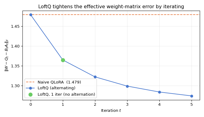 The dashed line is what QLoRA lives with forever. One SVD step (green) jumps most of the way down; the alternating loop (blue) keeps tightening from there. After about five iterations the curve stabilises - which is why the paper defaults to five.
A worked example: 3 × 3
Let’s trace the first iteration by hand with integer rounding standing in for NF4, so every step is verifiable. Consider:
\[W = \begin{bmatrix} 1.1 & 0.1 & 0.2 \\ 0.2 & 1.2 & 0.4 \\ 0.1 & 0.1 & 1.2 \end{bmatrix}\]Step 1 - initial quantization. Round every entry to the nearest integer:
\[Q_0 = \begin{bmatrix} 1 & 0 & 0 \\ 0 & 1 & 0 \\ 0 & 0 & 1 \end{bmatrix}, \qquad R_0 = W - Q_0 = \begin{bmatrix} 0.1 & 0.1 & 0.2 \\ 0.2 & 0.2 & 0.4 \\ 0.1 & 0.1 & 0.2 \end{bmatrix}\]The naive QLoRA error is $\|R_0\|_F = \sqrt{0.36} = 0.6$.
Step 2 - rank-1 SVD of the residual. Notice that $R_0$ factorises exactly:
\[R_0 = u \, v^T = \begin{bmatrix} 0.1 \\ 0.2 \\ 0.1 \end{bmatrix} \begin{bmatrix} 1 & 1 & 2 \end{bmatrix}\]so it’s already rank-1. With $r = 1$, LoftQ’s SVD sets $B_0 = u$ and $A_0 = v^T$, giving:
\[B_0 A_0 = R_0\]exactly. The residual after this step is zero - LoftQ has completely recovered $W$ at initialisation:
\[W_q + B_0 A_0 = Q_0 + R_0 = W\]Compare the three initial errors:
| Init strategy | $\Vert W - W_{\text{effective}} \Vert_F$ |
|---|---|
| Naive QLoRA ($B_0 = 0$) | 0.600 |
| LoftQ, 1 iteration | 0.000 |
| LoftQ, further iterations | 0.000 (already converged) |
This is a hand-picked case where the residual is exactly rank-1, which is why one step nails it. Real LLM layer residuals aren’t quite so generous - they’re high-rank with a dominant low-rank component. In that more realistic setting, one SVD iteration reduces but does not eliminate the error, and the alternation loop tightens it further with each pass. Empirically, five iterations are enough for the loop to stabilise.
What the numbers look like in practice
The LoftQ paper reports 2–5 % absolute accuracy recovery over QLoRA on GLUE at 4-bit - a modest but consistent gain. The more striking result is at 2-bit, where QLoRA’s naive init often fails to converge at all, while LoftQ still produces a trainable model. That’s the regime where “the adapter starts correct” stops being a nice-to-have and becomes the reason training works at all.
5. Comparison table
Before the row-by-row breakdown, here’s the whole training-state memory story for a 65B model in one picture:
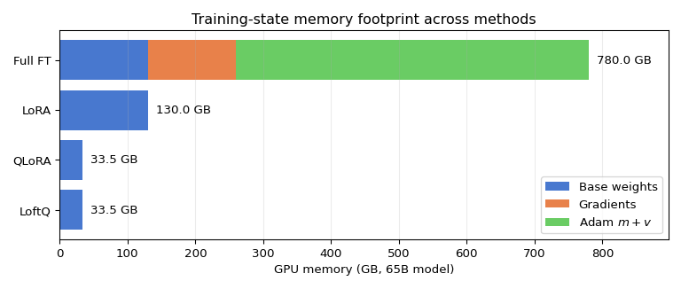 Full FT spends most of its memory on gradients and Adam states. LoRA keeps the base FP16 but drops those two bars entirely. QLoRA and LoftQ quantize the remaining base to NF4, landing around 33.5 GB - comfortably within a single 48 GB GPU.
| Full FT | LoRA | QLoRA | LoftQ | |
|---|---|---|---|---|
| Trainable params | 100 % | ~0.1 % | ~0.1 % | ~0.1 % |
| Base weights (65 B example) | 130 GB (FP16) | 130 GB (FP16) | 33.5 GB (NF4+DQ) | 33.5 GB (NF4+DQ) |
| Optimizer state | Scales with all params | Adapters only | Adapters only | Adapters only |
| Init quality at step 0 | Exact | Identical to base | Worse than base (by quant error) | Reduced init residual |
| Task accuracy vs Full FT | baseline | task-dependent, often close | a further task-dependent drop from base quantization | recovers more of that drop, most visibly at low bit-widths |
| Typical fit | Small models, or many GPUs | Medium models, full-precision-ready hardware | Large models on a single small GPU | Same as QLoRA, especially below 4-bit |
That accuracy row deliberately carries no fixed percentages: the gap depends on model, data, task, rank, target modules, optimizer, and quantization config, so any single “97%” would be folklore. The ordering is directional - each row buys memory and pays a task-dependent price - a measured trade, not a ranking. Rough guidance: LoftQ when accuracy matters at low bit-widths, QLoRA for most 4-bit work, plain LoRA when memory isn’t the binding constraint. Confirm on a representative eval.
6. The bigger picture
Let’s zoom out for a moment. The quantization series now has two halves:
- Inference-side toolkit - linear quantization, non-linear (NF4, quantile, k-means), and the smart-placement methods GPTQ and AWQ. All of these shrink an already-trained model for cheaper, faster serving.
- Training-side toolkit - LoRA, QLoRA, LoftQ. These shrink the training workflow itself, making enormous models fine-tunable on modest hardware.
It helps to place these methods against each other, and against true quantization-aware training, on the axes that actually differ - what the base does during training, what is trainable, and what the method is for:
| Method | Base during training | Trainable values | Main purpose |
|---|---|---|---|
| Full fine-tuning | full/selected precision, updated | all base parameters | maximum adaptation capacity |
| LoRA | frozen (full precision) | low-rank adapters | parameter-efficient adaptation |
| QLoRA | frozen, quantized (NF4), dequantized for compute | low-rank adapters | cut base storage during PEFT |
| LoftQ | frozen quantized base + jointly initialized adapter | adapters (after joint init) | reduce the initial quantization residual |
| QAT | simulated/actual low-precision path, updated | base and/or selected params | optimize the model’s behavior under quantization |
The bottom row is the one that gets conflated with the others: QAT trains the base through a low-precision path so the weights themselves become quantization-robust, whereas LoRA/QLoRA/LoftQ all keep the base frozen and only train adapters. Same neighbourhood, genuinely different mechanism.
The common thread across the training/inference halves is that useful weight updates and useful weight directions are low-entropy - concentrated near zero for weights, concentrated in a low-rank subspace for task-specific updates. Every method in the series exploits that concentration in some form:
- Non-linear grids spend bins where the weights actually live.
- GPTQ pushes errors into directions the Hessian says are cheap.
- AWQ protects the handful of channels that dominate the output.
- LoRA parametrises the update in the rank that actually matters.
- QLoRA quantizes what doesn’t change, and QLoRA + LoftQ starts the adapter at the right place.
NF4 showing up on both sides of the ledger - as an inference compression method and as the core of QLoRA’s training memory story - is the clearest evidence that “quantization for inference” and “quantization for training” aren’t separate fields. They’re the same few ideas applied to different halves of the model lifecycle.
If the inference-side counterpart isn’t fresh in mind yet, GPTQ and AWQ pick up where this article leaves off, with the uniform grid back in play and a different kind of cleverness in how weights land on it.
References
- LoRA: Low-Rank Adaptation of Large Language Models
- QLoRA: Efficient Finetuning of Quantized LLMs
- LoftQ: LoRA-Fine-Tuning-Aware Quantization for Large Language Models
Appendix A: Notation reference
| Symbol | Meaning |
|---|---|
| $W$ | Pre-trained weight matrix, shape $d_{out} \times d_{in}$ |
| $W_q$ | NF4-quantized base in QLoRA |
| $\Delta W$ | Fine-tuning update applied to $W$ |
| $A, B$ | LoRA adapter matrices; $A \in \mathbb{R}^{r \times d_{in}}$, $B \in \mathbb{R}^{d_{out} \times r}$ |
| $r$ | LoRA rank (typically 4–64) |
| $Q_t$ | LoftQ’s NF4 quantization at iteration $t$ |
| $R_t$ | LoftQ’s residual at iteration $t$: $R_t = W - Q_t$ |
| $U \Sigma V^T$ | SVD of the residual; top-$r$ components give the LoftQ initial adapter |
| DQ | Double Quantization - quantizing the NF4 scaling constants themselves |
Appendix B: LoRA in the broader PEFT landscape
LoRA is one of many parameter-efficient fine-tuning (PEFT) methods. The others are worth knowing by name even if a full walkthrough is beyond this article:
- Prefix / prompt tuning - prepend a small set of trainable “virtual tokens” to the input instead of modifying weights.
- Adapter tuning (Houlsby et al., 2019) - insert small trainable MLP bottlenecks between transformer layers. The original adapter paper; LoRA’s spiritual predecessor.
- IA³ - learn a small set of per-channel scaling factors rather than additive low-rank updates.
LoRA has become the dominant choice for large LLMs mainly because of the merging property: once training is done, $W + \frac{\alpha}{r}BA$ can be collapsed back into a full-precision base, so deployed models carry no extra adapter matmul (a quantized base needs the dequant/requant step discussed in §2). The other methods either can’t be merged cleanly or require extra runtime logic. LoRA also composes cleanly with quantization, as QLoRA and LoftQ demonstrate - which is why it’s the backbone of almost every practical low-cost fine-tuning recipe today.
Appendix C: A practical fine-tuning checklist
The memory tables above are arithmetic; a real run is reproducible only if the whole configuration is pinned and the measured peak memory is recorded, not just estimated. A workable checklist:
- Base model: exact model and revision/commit hash, plus license and its fine-tuning terms.
- Data and tokenizer: tokenizer / chat template, sequence length and whether examples are packed, the train/eval split, and a leakage check that eval data isn’t in the fine-tuning set.
- Adapter config: target modules (attention-only vs attention+MLP), rank $r$, scaling $\alpha$ (record $\alpha/r$), and adapter dropout.
- Quantization config (QLoRA/LoftQ): quant type (NF4), block/group size, double-quant on/off, and the compute dtype used for the dequantized matmul (BF16); for LoftQ, the number of alternating iterations and whether it’s the original or a library variant.
- Optimizer and schedule: optimizer (and whether it’s 8-bit/paged), learning rate and scheduler, gradient accumulation steps, and whether activation checkpointing is on.
- Measured cost: peak allocated and reserved VRAM (measured, e.g. via
torch.cuda.max_memory_allocated), throughput (tokens/s), and wall-clock time - not just the byte-counting estimate. - Quality: task metric with a baseline comparison (same-recipe full-precision LoRA, or full fine-tuning where feasible), so any quantization gap is quantified rather than assumed.
- Serving plan: adapter checkpoint, the merge-or-keep-separate decision (and, for a quantized base, whether merging is worth the numeric shift), and the serving kernel/format.
The non-negotiable line: measure peak memory and a baseline metric - the tables only get us to the ballpark; the run replaces the estimate with a real number.