From Boring to Brilliant: A Guide to LLM Sampling Techniques
- LLM sampling techniques You are here
- Temperature
- KV cache
- Prompt caching
- RAG evaluation
- Linear quantization
- Non-linear quantization
- AWQ
- GPTQ
- LoRA, QLoRA, and LoftQ
When we ask an LLM a question, it doesn’t just “know” the answer. At each step it produces a score for every possible next token, one step at a time. But how it turns those scores into an actual choice makes the difference between a robotic, repetitive answer and a creative, human-sounding response.
A quick word on “token” versus “word”: the model operates over tokens, and a token may be a whole word, part of a word, a punctuation mark, whitespace, or even raw bytes. We say “token” throughout, because that is the unit the algorithms below actually act on.
That final step, from a distribution over tokens to one emitted token, is the decoding policy, and this is a map of the common ones: what each does, how it trades off probability against diversity, latency, and repeatability, and where each fits. The one knob these methods lean on most, temperature, gets its own dedicated article; here we map the landscape, and that post goes deep on the softmax it all rests on.
1. The Deterministic Route: Searching for the “Best” Answer
These methods carry no intentional randomness: they try to score highly under the model’s own probabilities. A caution up front, though, because it is the single most common misconception about them: high model probability is not the same as correctness. These policies optimize what the model finds likely, not what is factually true, arithmetically right, or a good translation. Correctness has to come from the model itself, from grounding, from constraints, or from verification, never from the decoder alone.
A second caveat on “deterministic.” There is no sampling here, but “the same input always yields the same output” is still too strong in practice. Exact repeatability can depend on the serving stack, model version, numerical kernels, batching, and hardware, so treat determinism as “no intentional randomness,” not “bit-identical forever.”
Greedy Search
This is the simplest approach. At every step, the model strictly picks the single most probable next token (argmax). Crucially, that is a local choice: picking the best token now does not guarantee the most probable complete sentence, since an early high-probability token can lead into a lower-probability continuation than a different first token would have.
- Pros: It is fast, computationally cheap, and produces very coherent, on-topic text.
- Cons: It kills diversity. It is prone to getting stuck in repetitive loops (e.g., “I am I am I am…”) and is “brittle”: one locally-optimal token choice early on can derail the whole sentence.
- Best For: Reproducible baselines, extraction, and constrained formatting, where we want the same answer every time and low variance matters more than variety. (Reproducible is not the same as correct: a deterministic decoder will happily reproduce the same wrong answer.)
Beam Search
Think of this as a “smarter” Greedy Search. Instead of committing to the single best token at each step, it keeps track of the $k$ most probable partial sequences (called “beams”) simultaneously. Concretely, each step:
- expands every current partial sequence with candidate next tokens;
- scores the resulting longer sequences, commonly by their accumulated log-probability;
- keeps only the best $k$ active beams, discarding the rest;
- handles finished hypotheses (those that emit an end-of-sequence token) separately, setting them aside as completed candidates.
Two things are worth knowing. First, it is still only an approximation to the highest-probability sequence - once a path is discarded at step 3 it can never come back, so beam search can miss the true best sequence just as greedy can. Second, raw accumulated log-probability is a sum of negative numbers, so it favors shorter outputs (fewer terms to add up). Production beam search therefore applies a length normalization or length penalty to stop it from preferring truncated answers.
- Pros: It offers high fluency and is better at maintaining overall sequence logic than greedy.
- Cons: It is computationally expensive (roughly $k$ times the work) and can still result in generic, safe text.
- Best For: Machine translation and summarization, where the overall quality of the full sequence matters - though whether beam beats plain sampling is model- and task-dependent, not a given.
2. The Stochastic Route: Adding Diversity
To make text feel human, we introduce randomness (stochasticity). These methods sample from the probability distribution rather than always maximizing it - so even a low-probability token can be chosen, just rarely. The truncation methods below first cut the distribution down to a sensible pool, then sample from what remains.
Top-K Sampling
This method truncates the “tail” of the probability distribution. It keeps the top $k$ most probable tokens (e.g., the top 50), renormalizes their probabilities to sum to one, and samples from that pool.
- Pros: It balances diversity with coherence by filtering out “absurd” low-probability tokens.
- Cons: It isn’t adaptive. The cutoff $k$ is fixed. If the “true” list of good tokens is 3 but $k$ is 50, we might sample a bad one; if the list of good tokens is 200, we unfairly cut 150 of them.
- Best For: Creative tasks like story writing, chatbots, and brainstorming.
Top-P (Nucleus) Sampling
A common adaptive truncation strategy for open-ended generation. Instead of a fixed count of tokens, it keeps the smallest set of tokens whose cumulative probability reaches $p$ (e.g., $p=0.92$), renormalizes, and samples from that “nucleus.”
- Pros: The pool size adapts to the model’s confidence.
- If the model is certain (one token has 95% probability), the nucleus shrinks to just that token (behaving like greedy).
- If the model is uncertain, the nucleus expands to include many options.
- Best For: Open-ended chatbots, coding assistants, and creative writing. It is a frequent default, but “the default” varies by model and API and changes over time, so tune it rather than trusting a fixed number.
One distribution, three cuts
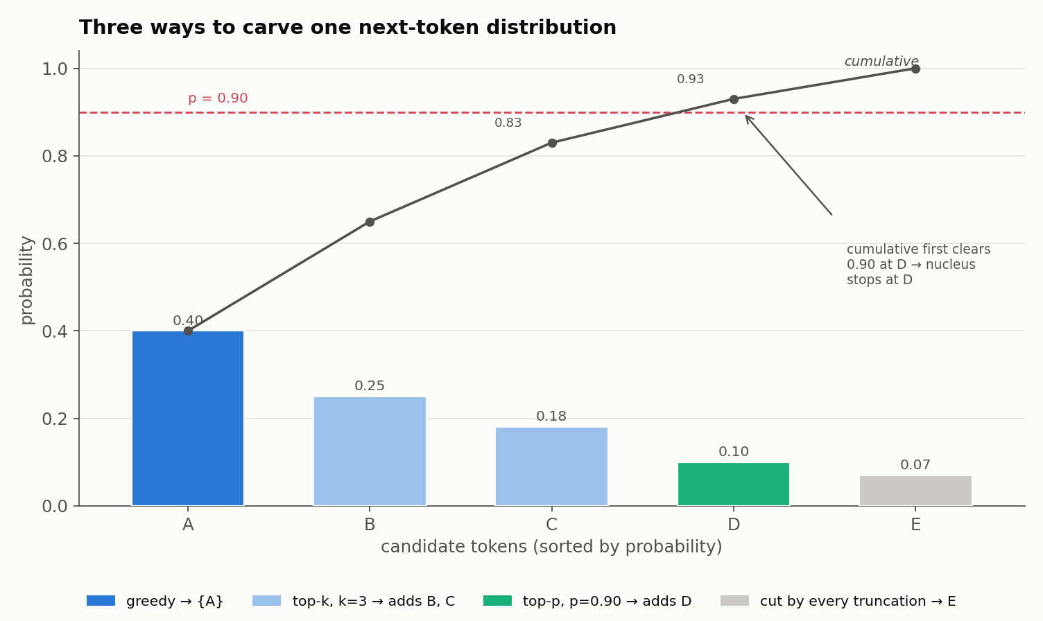
The cleanest way to see the difference is to fix a single next-token distribution and apply each policy to it. Say the model, at some step, produces:
| Token | A | B | C | D | E |
|---|---|---|---|---|---|
| Probability | 0.40 | 0.25 | 0.18 | 0.10 | 0.07 |
| Cumulative | 0.40 | 0.65 | 0.83 | 0.93 | 1.00 |
- Greedy takes the argmax: A, every time.
- Top-k, $k=3$ keeps the three most probable tokens, $\{A, B, C\}$.
- Top-p, $p=0.90$ walks the cumulative column until it reaches $0.90$: $A$ (0.40), then $+B$ (0.65), then $+C$ (0.83), then $+D$ (0.93 $\ge 0.90$). So the nucleus is $\{A, B, C, D\}$.
The step that is easy to miss is renormalization. After truncating, the surviving tokens no longer sum to one, so we rescale them - the excluded mass is redistributed, not deleted:
| Token | Original | Top-k ($k=3$) | Top-p ($p=0.90$) |
|---|---|---|---|
| A | 0.40 | 0.48 | 0.43 |
| B | 0.25 | 0.30 | 0.27 |
| C | 0.18 | 0.22 | 0.19 |
| D | 0.10 | - | 0.11 |
| E | 0.07 | - | - |
Two things this makes concrete. First, top-k and top-p can coincide on a given distribution (here they nearly do), but they diverge the moment the shape changes: sharpen the distribution and top-p’s nucleus shrinks toward greedy; flatten it and the nucleus grows - top-k, fixed at 3, cannot adapt either way. Second, because sampling draws from these renormalized pools, greedy’s confident “A” is only the most likely first token, not a guarantee about the best whole sentence - the same reason beam search hedges across several beams.
Deep Dive: Beam Search vs. Top-K Sampling
A common point of confusion is that both Beam Search and Top-K use a number “$k$.” However, they are fundamentally different tools for different jobs.
| Feature | Beam Search ($k=3$) | Top-K Sampling ($k=3$) |
|---|---|---|
| Type | Search Algorithm (Deterministic) | Sampling Method (Stochastic) |
| Goal | Approximate the most probable complete sequence | Pick one random, “good” next token |
| What is $k$? | Beam Width: Number of parallel sequences to track | Filter Size: Number of top tokens to choose from |
The “Cat” Example
Imagine the model is completing the sentence: “The cat sat on the…”
1. How Beam Search handles it ($k=2$) Beam search looks at the accumulated score of the entire sequence so far.
- It only keeps the top 2 partial paths: “The cat sat on the mat” and “The cat sat on the rug.” It permanently discards “floor” or “dog” - and cannot recover them later.
- It then explores the next token for those two specific paths to see which yields the highest total score for the full sequence.
- Result: No randomness, but only an approximation to the best path - because those discarded branches never come back, the true highest-probability sequence can slip through.
2. How Top-K handles it ($k=3$) Top-K makes a decision for right now, with no memory of other paths.
- It takes the top 3 tokens: mat (0.4), rug (0.3), floor (0.15).
- It renormalizes their probabilities to sum to 100% (mat becomes ~47%, rug ~35%, floor ~18%).
- It rolls the dice. There is a real chance it picks “rug” or “floor,” even if “mat” was the most likely.
- Result: Randomness is introduced. The model can produce something new.
How the Controls Compose
In practice these are rarely used one at a time. A typical decoding step chains several transforms, in roughly this order (an illustrative order - real libraries differ):
logits → penalties/constraints → temperature → truncation (top-k / top-p) → renormalize → sample
The order matters, because the controls interact:
- Temperature preserves ranking. A positive temperature rescales the logits but does not reorder them, so applying it before top-k does not change which tokens top-k keeps (the top 3 are still the top 3).
- But temperature changes top-p. Because it reshapes the cumulative masses, temperature shifts where the top-p nucleus stops - a hotter temperature flattens the distribution and grows the nucleus.
- Penalties and constraints re-rank. Repetition or frequency penalties, and hard constraints like grammars, can change the ordering itself, so they belong before truncation.
- A seed helps but does not guarantee. Fixing a random seed improves reproducibility but does not promise bit-identical output across different backends or hardware.
The softmax that temperature acts on is the subject of the temperature article; here it is enough to know where in the pipeline it sits.
Choosing a Starting Point
There is no universal “best” policy - only sensible starting points to tune on representative prompts. Treat the table as defaults to test, not folklore to trust:
| Goal | Useful starting point | What to evaluate |
|---|---|---|
| Reproducible baseline | Greedy or low-variance sampling | correctness, format adherence |
| Several candidate answers | Sampling, or beam variants | pass rate after reranking / verifying |
| Open-ended prose | Temperature + adaptive truncation (top-p) | diversity, coherence, repetition |
| Translation / summarization | Beam or sampling (model-dependent) | task metric + human preference |
| Structured output | Grammar / constrained decoding | schema validity + semantic accuracy |
Conclusion
Choosing a decoding policy is about matching the shape of the output to the task, not chasing a single “best” setting. Deterministic policies (greedy, beam) give reproducible, high-probability text - useful for baselines and constrained work, as long as we remember probability is not correctness. Stochastic policies (top-k, top-p, tuned with temperature) trade repeatability for the diversity that open-ended generation needs. The decoder shapes how the model speaks; getting a correct answer still depends on the model, its grounding, and how we verify it. The next article opens up the one control every stochastic policy leans on: temperature.