Same Ruler, Smarter Placement: GPTQ

In the previous article we saw how AWQ protects salient weight channels by pre-scaling them before INT4 rounding. The mechanism was direct: spend more of the grid’s resolution on the channels that meet loud activations, fold the inverse scale into the preceding layer, and standard hardware kernels keep working unchanged.

This article picks up the same problem from a different angle. GPTQ doesn’t try to pre-position the weights so they round cleanly. Instead, it rounds them one column at a time, measures the rounding error each step makes, and uses second-order information about the layer’s loss to push that error into the still-unquantized weights ahead of it. By the time the last column is processed, every prior mistake has been redistributed across the matrix in the direction that hurts the layer’s output least.

The 4×4 worked example, the layer-wise objective \(L(\hat W) = \|WX - \hat W X\|_F^2\), and the calibration magnitudes \(\mathbf{s}_X = [0.5, 4.0, 0.3, 0.2]^T\) all carry over from the AWQ article - so the two methods can be compared on identical input. Where AWQ adjusted weights before rounding via a per-channel scale, GPTQ adjusts them after rounding each one via the Hessian. Same starting equation, two different angles on it.

Refresher: this article leans on the Jacobian and Hessian throughout. If slope-and-curvature feels rusty, the companion Slope and Curvature primer builds both from scratch, including why GPTQ’s Hessian works out to exactly $2 X X^T$. Reading it first makes everything below easier.

---

1. GPTQ: The Error Compensator

1.1 The core idea in one sentence

When we round a weight to the nearest grid point, we create a small error. GPTQ uses second-order information (the Hessian of the layer-wise reconstruction loss \(\|WX - \hat W X\|_F^2\), not the end-to-end training loss) to figure out the optimal way to nudge the remaining weights so they absorb that error before they themselves are quantized. This distinction matters throughout: everything below is curvature of a local, per-layer objective computed from calibration activations, never the model’s global loss surface.

A useful mental picture: think of packing a suitcase. Each time we put an item in (quantize a column), we rearrange the remaining contents (update the unquantized columns) so the rest still fits well. By the time the last column goes in, every prior rounding error has been spread out as gently as possible across everything that came after it.

1.2 A short family tree

GPTQ didn’t come from nowhere. It descends from two earlier ideas:

• Optimal Brain Surgeon (Hassibi & Stork, 1993), used a second-order Taylor expansion of the loss to derive the optimal compensating update when one weight is pruned to zero. The math was clean, but the original setting was network pruning, not quantization.
• Optimal Brain Quantization (OBQ; Frantar & Alistarh, 2022), extended the same closed form from pruning to rounding. Greedily picks the weight whose quantization causes the least damage, quantizes it, updates the rest, repeats. Mathematically elegant but far too slow at scale, OBQ is $O(d_{out} \cdot d_{in}^3)$ per layer, which is out of the question for a 70B model.

GPTQ (Frantar et al., 2022) contributes not new math but three engineering moves that turn the same core idea into an $O(d_{out} \cdot d_{in}^2)$ algorithm:

1. A fixed column order instead of greedy selection.
2. Block-wise lazy updates that convert many tiny column ops into one fat matmul.
3. A Cholesky-based precomputation that collapses the whole update schedule into one triangular matrix.

The rest of this section unpacks each piece.

1.3 Second-order information in one picture

Before any Hessian math, here’s the intuition in a single picture. Imagine the layer’s output error as a bowl sitting on top of the trained weights. Along some weight directions the bowl is shallow, we can shift that weight a lot and the output barely moves. Along others it is steep, a tiny shift causes a lot of damage.

The Hessian is the curvature map of that bowl (again, the bowl of the layer reconstruction error, not the model’s training loss). First-order information (the gradient) tells us the slope at a single point; second-order information tells us how the slope changes as we walk in every direction. Here the gradient is not the useful signal: the reconstruction bowl is centred at $\hat W = W$ (zero error), so what governs the damage of a rounding step is purely the curvature of that bowl. The curvature tells us exactly how expensive each direction is, and the inverse curvature tells us where to push other weights so they can absorb the cost.

1.4 Where does $H = 2 X X^T$ come from?

Recall the layer-wise objective from the AWQ article:

\[L(\hat W) \;=\; \| W X - \hat W X \|_F^2\]

Writing $\delta W = \hat W - W$ for the perturbation:

\[L(\delta W) \;=\; \| \delta W \cdot X \|_F^2\]

We want the Hessian of $L$ with respect to each row of $\delta W$. Let’s derive this step by step rather than waving at “differentiating a quadratic.”

Pick a single row $r$ of $\delta W$, call it \(\mathbf{v}_r \in \mathbb{R}^{d_{in}}\) as a column vector (so \(\mathbf{v}_r^T\) is the corresponding row of $\delta W$). The contribution of this row to the Frobenius norm is the row-wise sum of squared entries of $\delta W \cdot X$. Since matrix-multiplication acts independently across rows (row $r$ of $\delta W \cdot X$ equals \(\mathbf{v}_r^T X\), depending only on \(\mathbf{v}_r\)), we can split $L$ by rows:

\[L(\delta W) \;=\; \sum_{r=0}^{d_{out}-1} \|\mathbf{v}_r^T X\|_2^2\]

Expand one row’s contribution. Let \(\mathbf{a} = X^T \mathbf{v}_r\) (a column vector of length $n_{samples}$). Then \(\mathbf{v}_r^T X = \mathbf{a}^T\), and

\[\|\mathbf{v}_r^T X\|_2^2 \;=\; \mathbf{a}^T \mathbf{a} \;=\; (X^T \mathbf{v}_r)^T (X^T \mathbf{v}_r) \;=\; \mathbf{v}_r^T \, X X^T \, \mathbf{v}_r\]

So each row’s contribution is a quadratic form \(\mathbf{v}_r^T (X X^T) \mathbf{v}_r\) in \(\mathbf{v}_r\), with the same matrix $X X^T$ for every row. For a quadratic form $f(\mathbf{v}) = \mathbf{v}^T M \mathbf{v}$ with $M$ symmetric, the Hessian is $\nabla^2 f = 2 M$. We can verify by writing out indices:

\[f(\mathbf{v}) \;=\; \sum_{j,k} M_{jk} v_j v_k, \qquad \frac{\partial f}{\partial v_i} \;=\; 2 \sum_k M_{ik} v_k, \qquad \frac{\partial^2 f}{\partial v_i \, \partial v_{i'}} \;=\; 2 M_{i i'}\]

So the Hessian of the row contribution is \(\nabla^2_{\mathbf{v}_r} f = 2 \, X X^T\). And because $X X^T$ doesn’t depend on $r$, it’s the same Hessian for every row:

\[H \;=\; 2 \, X X^T\]

Two observations are worth pausing on:

• $H$ has shape $d_{in} \times d_{in}$, it’s indexed by input channels, not output channels. Each entry $H_{jk}$ measures coupling between input channel $j$ and input channel $k$ in the calibration data.
• $X X^T$ is the input Gram matrix, the uncentred second moment of the calibration inputs (it is proportional to the covariance only if the activations are mean-centred, which they generally are not, so “second moment” is the accurate term). Its diagonal entries \([X X^T]_{jj} = \sum_t X_{j,t}^2\) measure how loudly each input channel fires on average. Its off-diagonals \([X X^T]_{jk} = \sum_t X_{j,t} X_{k,t}\) measure how channels co-fire.

Reading the Hessian this way: weights on loud, strongly-correlated channels are expensive to mis-round, because their errors cascade through the dot product and collide instead of averaging out; weights on quiet, independent channels are cheap. So we compute $H$ once per layer from calibration data and reuse it across all $d_{out}$ rows of $W$.

1.5 The closed-form compensating update

Now we have everything we need to write down GPTQ’s per-column update.

Suppose we’ve just quantized column $q$ of the weight matrix: we replaced $W_{:,q}$ with $\hat W_{:,q} = \text{quant}(W_{:,q})$. The rounding error in that column is

\[e_q \;=\; W_{:,q} - \hat W_{:,q} \qquad (\text{shape } d_{out} \times 1)\]

This rounding choice is now fixed; we can’t change it. But we can compensate by adjusting all the unquantized columns $q+1, q+2, \ldots, d_{in}-1$ so that the layer’s output, with the modified weights, stays as close as possible to the original output.

For each row $r$ of $W$, write the row vector as \(\mathbf{w}_r\). The layer-wise reconstruction error is, up to constants, the quadratic $\frac{1}{2} \boldsymbol{\delta}^T H \boldsymbol{\delta}$ in the perturbation \(\boldsymbol{\delta} = \mathbf{w}_r^{\text{new}} - \mathbf{w}_r^{\text{orig}}\). Minimising $\frac{1}{2} \boldsymbol{\delta}^T H \boldsymbol{\delta}$ subject to the constraint that the $q$-th entry $\delta_q$ is fixed at a known value gives (via Lagrange multipliers; the Slope and Curvature primer covers the second-order machinery) a closed-form solution:

\[\delta_j^* \;=\; \frac{\delta_q}{[H^{-1}]_{qq}} \, [H^{-1}]_{q,j} \qquad \text{for } j \ne q\]

With $\delta_q = \hat w_q - w_q^{\text{orig}} = -e_q$ (the change forced by quantization), this becomes:

\[\delta_j^* \;=\; -\frac{e_q}{[H^{-1}]_{qq}} \, [H^{-1}]_{q,j}\]

So the optimal new weight is \(\mathbf{w}^{\text{new}}_j = \mathbf{w}^{\text{orig}}_j + \delta_j^* = \mathbf{w}^{\text{orig}}_j - \frac{e_q}{[H^{-1}]_{qq}} [H^{-1}]_{q,j}\). Applied across all output rows (vectorising over $r$) and all unquantized columns ($j > q$), we get the three update steps:

Step 1: Quantize the current column:

\[\hat W_{:,q} \;=\; \text{quant}(W_{:,q})\]

Step 2: Compute the normalised error (per row):

\[\mathbf{err}_{:,q} \;=\; \frac{W_{:,q} - \hat W_{:,q}}{[H^{-1}]_{qq}}\]

Step 3: Compensate the remaining columns by pushing the error along the row of $H^{-1}$:

\[W_{:, \, q+1:} \;\mathrel{-}= \; \mathbf{err}_{:,q} \cdot \big[H^{-1}\big]_{q, \, q+1:}\]

Three pieces of intuition for these formulas, one for each piece:

• $W_{:,q} - \hat W_{:,q}$ is “the mistake I just made by rounding this column,” one entry per output row.
• \(\big/ [H^{-1}]_{qq}\) normalises the raw mistake by the direction’s conditional curvature. To be precise about which matrix does what: $H$ is the curvature, and the effective (conditional) curvature of column $q$ after earlier columns are fixed is \(1/[H^{-1}]_{qq}\); the entry \([H^{-1}]_{qq}\) itself is its inverse (a “compliance”). We use “stiffness” loosely for \(1/[H^{-1}]_{qq}\). A stiff direction (large curvature, hence small \([H^{-1}]_{qq}\)) is under heavy spring tension, so a small mis-round there implies a large restoring force; dividing by \([H^{-1}]_{qq}\) turns the error into a unit-less quantity we can spread around.
• \(\times \; [H^{-1}]_{q, \, q+1:}\) is “spread that force across the remaining columns, in exactly the direction where they are coupled enough to absorb it best.” The off-diagonal entries of $H^{-1}$ encode the coupling between input channels.

That last step is the crux: it pushes each row’s quantization error into the still-unquantized weights, so every subsequent rounding decision is informed by all prior errors, and by the last column those errors have been absorbed.

Importantly, one specific step here is exact: because the layer-wise reconstruction objective is exactly quadratic (we showed this in the AWQ article), the compensating update solves “given the rounding decision at column $q$, what nudge to the remaining weights best preserves this layer’s calibration output?” exactly, not approximately. That is a real and useful property. It is worth being precise about scope, though, because “GPTQ approximates nothing” would badly oversell it. GPTQ makes several approximations that all matter in practice:

• it optimises layer-wise reconstruction on calibration data, a proxy for the end-to-end task loss, not the loss itself;
• the Hessian is estimated from finite calibration data, so it is a sample estimate;
• it adds damping ($\lambda I$), which regularises the solution away from the raw optimum;
• it fixes a column order (a heuristic, even with act-order) rather than searching orderings jointly;
• it depends on the chosen quantizer, group size, and scale/clip policy;
• it does no cross-layer compensation - each layer is quantized in isolation, so errors are not reconciled across the network.

What is exact is the per-column compensation sub-problem given all the choices above. Everything wrapped around it is an approximation, and a good one empirically, but the honest statement is “exact sub-problem inside an approximate pipeline,” not “approximates nothing except sequential processing.”

1.6 Dampening: keeping the math stable

Before inverting the Hessian, GPTQ adds a small diagonal perturbation:

\[H_{\text{damp}} \;=\; H + \lambda \, I, \qquad \lambda \;=\; 0.01 \cdot \overline{\text{diag}(H)}\]

(the dampening constant $\lambda$ is $1\%$ of $H$’s average diagonal). This serves three purposes.

Purpose 1: Numerical positive-definiteness. Calibration data may be rank-deficient (e.g., if some input channels never fire in the calibration set, their corresponding rows/columns of $X X^T$ are zero, making $H$ singular). Adding $\lambda I$ shifts every eigenvalue of $H$ upward by $\lambda$. Concretely, if $H = U \, \text{diag}(\mu_1, \ldots, \mu_n) \, U^T$ is the eigendecomposition (with $U$ orthogonal), then

\[H + \lambda I \;=\; U \, \text{diag}(\mu_1 + \lambda, \ldots, \mu_n + \lambda) \, U^T\]

, same eigenvectors, every eigenvalue increased by $\lambda$. If some $\mu_i$ were zero (or negative due to floating-point noise), they become $\lambda > 0$, and the matrix is now strictly positive definite. Cholesky decomposition (which we use in the next subsection) requires positive-definiteness, so this is non-optional.

Purpose 2: Bounded compensation magnitudes. The update factor in Step 3 above involves dividing by \([H^{-1}]_{qq}\). Suppose $H$ has a very small eigenvalue near zero in the direction of column $q$. Then $H^{-1}$ has a very large eigenvalue there, and \([H^{-1}]_{qq}\) becomes huge. That makes the “normalised force” \(\mathbf{err}_{:,q} / [H^{-1}]_{qq}\) tiny. Meanwhile, the update vector \([H^{-1}]_{q, q+1:}\) becomes huge. The two don’t perfectly cancel in practice, and the result is numerically unstable.

After dampening, the smallest eigenvalue of $H_{\text{damp}}$ is at least $\lambda$, so the largest eigenvalue of $H_{\text{damp}}^{-1}$ is at most $1/\lambda$. In particular, every diagonal entry \([H_{\text{damp}}^{-1}]_{qq}\) is bounded:

\[[H_{\text{damp}}^{-1}]_{qq} \;=\; \mathbf{e}_q^T H_{\text{damp}}^{-1} \mathbf{e}_q \;\le\; \|H_{\text{damp}}^{-1}\|_2 \;=\; \frac{1}{\mu_{\min}(H_{\text{damp}})} \;\le\; \frac{1}{\lambda}\]

(the first inequality holds because for any positive-definite $M$ and unit vector $\mathbf{e}$, \(\mathbf{e}^T M \mathbf{e} \le \|M\|_2\), the largest eigenvalue). So dampening puts a hard cap on how aggressive the compensation can get.

Purpose 3: Gentle regularisation. Beyond numerical safety, dampening acts as a Tikhonov-style regulariser, it biases the closed-form solution slightly toward “do less compensation,” which prevents overfitting to noise in the calibration data. The choice $\lambda = 0.01 \cdot \overline{\text{diag}(H)}$ (1% of the mean diagonal) is the GPTQ reference implementation’s default percdamp, chosen empirically to be small enough to barely affect the dominant directions of $H$ yet large enough to tame nearly-degenerate ones; it is a sensible default, not a universal constant, and some models need it tuned.

1.7 The Cholesky trick, derived

This is the most elegant piece of GPTQ, and the most often glossed over. Deriving it makes the engineering story (precompute once, read updates off row by row) obvious rather than magical.

The setup. When we quantize column $q$ and want to compute the optimal compensation for column $j > q$, the original $H^{-1}$ isn’t quite right. We need the conditional inverse Hessian, given that columns $0, 1, \ldots, q$ have already been fixed. Mathematically, after fixing column $q$, the inverse Hessian for the remaining problem (columns $q+1, q+2, \ldots$) is the Schur complement:

\[\big[H^{-1}\big]_{\text{cond}}^{(q+1:)} \;=\; \big[H^{-1}\big]_{q+1:,\, q+1:} \;-\; \frac{\big[H^{-1}\big]_{q+1:,\, q} \cdot \big[H^{-1}\big]_{q,\, q+1:}}{\big[H^{-1}\big]_{qq}}\]

This formula updates the inverse Hessian to reflect the new conditional structure. In the original OBQ, this is exactly the rank-one update applied after each weight is quantized. The cost is $O(d_{in}^2)$ per column, summing to $O(d_{in}^3)$ per row. That’s what makes OBQ too slow at scale.

The observation. GPTQ spots something elegant. The sequence of “compute conditional inverse, use its first row to update the rest, eliminate first row/column, repeat” is exactly what Cholesky decomposition computes. And it gives it to us for free, in a single $O(d_{in}^3)$ precomputation.

The derivation for a 2×2 case. Take $H^{-1}$ as a $2 \times 2$ symmetric positive-definite matrix $\begin{bmatrix} a & b \ b & c \end{bmatrix}$, and write the upper-triangular Cholesky factor $U$ such that $H^{-1} = U^T U$:

\[U \;=\; \begin{bmatrix} u_{00} & u_{01} \\ 0 & u_{11} \end{bmatrix}\]

Then $U^T U = \begin{bmatrix} u_{00}^2 & u_{00} u_{01} \ u_{00} u_{01} & u_{01}^2 + u_{11}^2 \end{bmatrix}$, which must equal $\begin{bmatrix} a & b \ b & c \end{bmatrix}$. Solving:

\[u_{00} \;=\; \sqrt{a}, \qquad u_{01} \;=\; \frac{b}{\sqrt{a}}, \qquad u_{11} \;=\; \sqrt{c - \frac{b^2}{a}}\]

Now compute the ratio:

\[\frac{u_{01}}{u_{00}} \;=\; \frac{b / \sqrt{a}}{\sqrt{a}} \;=\; \frac{b}{a} \;=\; \frac{[H^{-1}]_{01}}{[H^{-1}]_{00}}\]

This is exactly the GPTQ update factor for column 1 when column 0 is being quantized. And $u_{11}^2 = c - b^2/a$ is the Schur complement \([H^{-1}]_{\text{cond}}^{(1)}\), exactly the conditional inverse Hessian for the remaining problem.

The general pattern. This generalises: row $q$ of the upper-triangular Cholesky factor $U$ of $H^{-1}$ encodes everything we need for the $q$-th quantization step.

• $u_{qq}^2$ equals the effective \([H_{\text{cond}}^{-1}]_{qq}\) after the first $q$ columns have been eliminated, the diagonal stiffness in the conditional problem at step $q$.
• $u_{q, j} / u_{qq}$ for $j > q$ equals \([H_{\text{cond}}^{-1}]_{qj} / [H_{\text{cond}}^{-1}]_{qq}\) at step $q$, exactly the update factor for column $j$ when column $q$ is being quantized.

(The mechanical proof of the general case follows by induction, using the fact that the Cholesky factor of the Schur complement of $H^{-1}$ at row $q$ is precisely $U[q+1:, q+1:]$. The 2×2 case above contains the whole flavour.)

The payoff. OBQ does an $O(d_{in}^2)$ rank-one update after each column, totalling $O(d_{in}^3)$ for $d_{in}$ columns. GPTQ takes a different route. It computes $U$ once at the start in $O(d_{in}^3)$ time. From there, every update vector can be read directly off the rows of $U$. The total schedule of compensations is precomputed, baked into one upper-triangular matrix. No further Hessian updates are needed during the actual quantization sweep.

In code, this is exactly four steps:

H = H + damp * torch.eye(d_in)                # 1. dampening
H_chol = torch.linalg.cholesky(H)             # 2. Cholesky of H
Hinv = torch.cholesky_inverse(H_chol)         # 3. H^{-1} via Cholesky
U = torch.linalg.cholesky(Hinv, upper=True)   # 4. upper-tri Cholesky of H^{-1}

After this, $u_{qq}$ and $u_{q, q+1:}$ (the rows of $U$) give all the information needed for the column-by-column quantization sweep. No matrix updates inside the loop; just reads from $U$ and per-row arithmetic on $W$.

1.8 The lazy batch update (block size = 128)

Processing one column at a time is correct but slow on real hardware; each step touches only a single column of $W$, which underutilises the GPU’s matmul throughput. GPTQ groups columns into blocks (typically 128 columns per block) and amortises the compensation work:

for each block [i1, i2) of 128 columns:
    for each column q within the block:
        1. quantize column q
        2. update only the remaining columns WITHIN this block (q+1 to i2-1)
           - accumulate the compensation but DON'T apply it to future blocks yet
    after the block is done:
        3. apply the accumulated error from all 128 columns to ALL future columns
           in a single large matmul

Step 3 is the key: it converts many tiny column updates (each of size $d_{out} \times (\text{remaining cols outside block})$) into one large matmul of size $d_{out} \times 128 \times (\text{cols outside block})$. GPUs eat large matmuls for breakfast, so this is what makes GPTQ fast enough for billion-parameter models: the GPTQ paper reports quantizing the largest OPT/BLOOM models (~175B) in roughly four GPU-hours, with smaller models correspondingly faster. Exact times depend on hardware, model, and calibration size, so treat these as order-of-magnitude figures.

The numerical result is mathematically identical to processing columns one at a time; lazy batching only changes when updates are applied, not what updates are applied.

1.9 Activation ordering (actorder)

An optional enhancement called activation ordering (often surfaced as desc_act in quantization libraries) sorts columns by decreasing Hessian diagonal before quantizing:

\[\text{perm} \;=\; \text{argsort}\big(\text{diag}(H), \; \text{descending}\big)\]

Recall \([H]_{jj} = 2 \sum_t X_{j,t}^2\) measures how sensitive the output is to weights in column $j$ (loud channels have high diagonal entries). By quantizing the most sensitive columns first, they get the maximum number of remaining columns available for error compensation. Less sensitive columns are quantized later with fewer compensating degrees of freedom, but they need less compensation anyway, because their errors hurt less.

Actorder typically improves quantization quality by 0.1–0.5 perplexity points on standard LLM benchmarks. It’s a free win in accuracy, at a small cost in implementation complexity: we need to permute the weight matrix and remember to permute the activations correspondingly at inference time.

1.10 Complexity

Putting all the pieces together, the cost breakdown per layer is:

Step	Cost
Hessian computation: $H = 2 X X^T$	$O(d_{in}^2 \cdot n_{samples})$
Dampening + double Cholesky precomputation	$O(d_{in}^3)$
Column-by-column quantization (all rows, block-batched)	$O(d_{out} \cdot d_{in}^2)$
Total per layer	$O\big(\max(\,d_{out} \cdot d_{in}^2, \; d_{in}^3\,)\big)$

Compare to OBQ’s $O(d_{out} \cdot d_{in}^3)$: GPTQ saves a full factor of $d_{in}$, which is the difference between “weeks” and “hours” for a 70B model.

1.11 Step-by-step on the 4×4 example

Now we apply GPTQ to the same matrix we used for AWQ. To make this work as a hand-traceable example, we need a plausible Hessian $H = 2 X X^T$. We don’t have real calibration activations to compute it from. So we’ll write down one that’s consistent with the calibration magnitudes \(\mathbf{s}_X = [0.5, 4.0, 0.3, 0.2]^T\). Suppose:

\[H \;\approx\; \begin{bmatrix} \phantom{-}2.0 & 0.5 & 0.1 & 0.2 \\ \phantom{-}0.5 & 8.0 & 0.3 & 0.4 \\ \phantom{-}0.1 & 0.3 & 1.5 & 0.2 \\ \phantom{-}0.2 & 0.4 & 0.2 & 1.0 \end{bmatrix}\]

Two things to notice in $H$:

• $H_{11} = 8.0$, the diagonal for input channel 1 is much larger than the others. This is consistent with \(\mathbf{s}_X\): channel 1 fires with magnitude 4, so $\sum_t X_{1,t}^2$ is large.
• Off-diagonal entries are small but non-zero; input channels are slightly correlated, but mostly independent.

Inverting $H$ (after dampening, which we’ll absorb into the rounded values below):

\[H^{-1} \;\approx\; \begin{bmatrix} \phantom{-}0.52 & -0.03 & -0.02 & -0.09 \\ -0.03 & \phantom{-}0.13 & -0.02 & -0.04 \\ -0.02 & -0.02 & \phantom{-}0.69 & -0.13 \\ -0.09 & -0.04 & -0.13 & \phantom{-}1.06 \end{bmatrix}\]

(Rounded to 2 decimals for readability. We can verify approximately that $H H^{-1} \approx I$.)

The diagonal entries \([H^{-1}]_{jj}\) are the stiffnesses we’ll divide by, and the off-diagonals \([H^{-1}]_{q, q+1:}\) are the spreading vectors. Notice that \([H^{-1}]_{11} = 0.13\) is the smallest, corresponding to the stiffest direction, which is exactly the salient channel 1 (high curvature, hard to mis-round). Conversely, \([H^{-1}]_{33} = 1.06\) is the largest, corresponding to the shallowest direction (channel 3 fires very rarely, so errors there cost little).

We’ll quantize column-by-column with per-column INT4 scales (each column gets \(\Delta_q = \max\lvert W_{:,q}\rvert / 7\) where the max is taken over the current, possibly already-updated column).

Column 0

Original column 0: $[0.10, -0.20, 0.40, -0.15]$.

• \(\max\lvert\cdot\rvert = 0.40\), scale $\Delta_0 = 0.40/7 \approx 0.0571$.
• Codes: $\text{round}(W_{:,0} / \Delta_0)$:
  • $0.10 / 0.0571 \approx 1.75 \to 2$
  • $-0.20 / 0.0571 \approx -3.50 \to -4$ (half rounds away from zero)
  • $0.40 / 0.0571 \approx 7.00 \to 7$
  • $-0.15 / 0.0571 \approx -2.63 \to -3$
• Codes: $[2, -4, 7, -3]$.
• Dequant: $[2, -4, 7, -3] \cdot 0.0571 \approx [0.1143, -0.2286, 0.4000, -0.1714]$.
• Error $e_0 = W_{:,0} - \hat W_{:,0} \approx [-0.0143, \,+0.0286, \,0.0000, \,+0.0214]$.

Now compensate columns 1, 2, 3 using row 0 of $H^{-1}$. The update for column $j$ is

\[W_{:,j} \;\mathrel{-}= \; \frac{e_0}{[H^{-1}]_{00}} \cdot [H^{-1}]_{0,j}\]

Define the compensation factor \(f_{0 \to j} = [H^{-1}]_{0,j} / [H^{-1}]_{00}\):

• $f_{0 \to 1} = -0.03 / 0.52 \approx -0.0577$
• $f_{0 \to 2} = -0.02 / 0.52 \approx -0.0385$
• $f_{0 \to 3} = -0.09 / 0.52 \approx -0.1731$

Compute the per-row increment to subtract for each column: $e_0 \cdot f_{0 \to j}$.

• For column 1: $e_0 \cdot (-0.0577) \approx [+0.00083, -0.00165, 0, -0.00124]$. Subtracting from column 1: $[2.50 - 0.00083, 3.20 + 0.00165, -2.80, 2.10 + 0.00124] \approx [2.4992, 3.2017, -2.8000, 2.1012]$.
• For column 2: $e_0 \cdot (-0.0385) \approx [+0.00055, -0.00110, 0, -0.00082]$. New column 2 $\approx [-0.3006, 0.1511, 0.2500, -0.3992]$.
• For column 3: $e_0 \cdot (-0.1731) \approx [+0.00247, -0.00495, 0, -0.00371]$. New column 3 $\approx [0.0475, -0.0751, 0.1200, 0.0637]$.

After column 0 (replaced with its dequant, columns 1–3 compensated):

\[W^{(1)} \;\approx\; \begin{bmatrix} \phantom{-}0.1143 & \phantom{-}2.4992 & -0.3006 & \phantom{-}0.0475 \\ -0.2286 & \phantom{-}3.2017 & \phantom{-}0.1511 & -0.0751 \\ \phantom{-}0.4000 & -2.8000 & \phantom{-}0.2500 & \phantom{-}0.1200 \\ -0.1714 & \phantom{-}2.1012 & -0.3992 & \phantom{-}0.0637 \end{bmatrix}\]

Column 1

Adjusted column 1: $[2.4992, 3.2017, -2.8000, 2.1012]$.

• \(\max\lvert\cdot\rvert = 3.2017\), scale $\Delta_1 = 3.2017/7 \approx 0.4574$.
• Codes:
  • $2.4992 / 0.4574 \approx 5.46 \to 5$
  • $3.2017 / 0.4574 \approx 7.00 \to 7$
  • $-2.8000 / 0.4574 \approx -6.12 \to -6$
  • $2.1012 / 0.4574 \approx 4.59 \to 5$
• Codes: $[5, 7, -6, 5]$.
• Dequant: $[5, 7, -6, 5] \cdot 0.4574 \approx [2.2869, 3.2017, -2.7443, 2.2869]$.
• Error $e_1 \approx [+0.2123, \,0.0000, \,-0.0557, \,-0.1857]$.

Compensation factors for remaining columns 2, 3 (using row 1 of $H^{-1}$):

• $f_{1 \to 2} = -0.02 / 0.13 \approx -0.1538$
• $f_{1 \to 3} = -0.04 / 0.13 \approx -0.3077$

Increments to subtract:

• Column 2: $e_1 \cdot (-0.1538) \approx [-0.0327, 0, +0.00857, +0.02856]$. New column 2 $\approx [-0.3006 - (-0.0327), 0.1511 - 0, 0.2500 - 0.00857, -0.3992 - 0.02856] \approx [-0.2679, 0.1511, 0.2414, -0.4278]$.
• Column 3: $e_1 \cdot (-0.3077) \approx [-0.0653, 0, +0.01714, +0.05713]$. New column 3 $\approx [0.0475 - (-0.0653), -0.0751 - 0, 0.1200 - 0.01714, 0.0637 - 0.05713] \approx [0.1128, -0.0751, 0.1029, 0.0066]$.

After column 1:

\[W^{(2)} \;\approx\; \begin{bmatrix} \phantom{-}0.1143 & \phantom{-}2.2869 & -0.2679 & \phantom{-}0.1128 \\ -0.2286 & \phantom{-}3.2017 & \phantom{-}0.1511 & -0.0751 \\ \phantom{-}0.4000 & -2.7443 & \phantom{-}0.2414 & \phantom{-}0.1029 \\ -0.1714 & \phantom{-}2.2869 & -0.4278 & \phantom{-}0.0066 \end{bmatrix}\]

The interesting row here is row 0: original $w_{0,1} = 2.50$, naive rounding would have sent it to $\text{quant}(2.50) = 5$ at scale $0.4574 \to \hat w = 2.287$, an error of $0.213$. GPTQ’s compensation from column 0 nudged $w_{0,1}$ down to $2.4992$ first. That still rounds to $5$. But now the residual error $+0.2123$ gets propagated forward into columns 2 and 3, so subsequent rounding decisions are aware of it.

Column 2

Adjusted column 2: $[-0.2679, 0.1511, 0.2414, -0.4278]$.

• \(\max\lvert\cdot\rvert = 0.4278\), scale $\Delta_2 = 0.4278/7 \approx 0.0611$.
• Codes:
  • $-0.2679 / 0.0611 \approx -4.39 \to -4$
  • $0.1511 / 0.0611 \approx 2.47 \to 2$
  • $0.2414 / 0.0611 \approx 3.95 \to 4$
  • $-0.4278 / 0.0611 \approx -7.00 \to -7$
• Codes: $[-4, 2, 4, -7]$.
• Dequant: $[-4, 2, 4, -7] \cdot 0.0611 \approx [-0.2444, 0.1222, 0.2444, -0.4278]$.
• Error $e_2 \approx [-0.0235, \,+0.0289, \,-0.0030, \,0.0000]$.

Compensation factor for column 3 (last unquantized column):

• $f_{2 \to 3} = -0.13 / 0.69 \approx -0.1884$

Increment: $e_2 \cdot (-0.1884) \approx [+0.00443, -0.00544, +0.000565, 0]$. New column 3:

• $[0.1128 - 0.00443, -0.0751 - (-0.00544), 0.1029 - 0.000565, 0.0066 - 0]$
• $\approx [0.1084, -0.0696, 0.1023, 0.0066]$.

Column 3 (final, no further compensation)

Adjusted column 3: $[0.1084, -0.0696, 0.1023, 0.0066]$.

• \(\max\lvert\cdot\rvert = 0.1084\), scale $\Delta_3 = 0.1084/7 \approx 0.0155$.
• Codes:
  • $0.1084 / 0.0155 \approx 7.00 \to 7$
  • $-0.0696 / 0.0155 \approx -4.49 \to -4$
  • $0.1023 / 0.0155 \approx 6.60 \to 7$
  • $0.0066 / 0.0155 \approx 0.43 \to 0$
• Codes: $[7, -4, 7, 0]$.
• Dequant: $[7, -4, 7, 0] \cdot 0.0155 \approx [0.1084, -0.0620, 0.1084, 0.0000]$.

Final GPTQ-quantized matrix

Assembling all four columns’ dequantized values:

\[\hat W^{\text{GPTQ}} \;\approx\; \begin{bmatrix} \phantom{-}0.1143 & \phantom{-}2.2869 & -0.2444 & \phantom{-}0.1084 \\ -0.2286 & \phantom{-}3.2017 & \phantom{-}0.1222 & -0.0620 \\ \phantom{-}0.4000 & -2.7443 & \phantom{-}0.2444 & \phantom{-}0.1084 \\ -0.1714 & \phantom{-}2.2869 & -0.4278 & \phantom{-}0.0000 \end{bmatrix}\]

Compare this to $\hat W^{\text{naive}}$ from the AWQ article. The differences are striking:

• Column 0 is now non-trivially populated (codes $[2, -4, 7, -3]$ at per-column scale $0.0571$, where naive per-tensor rounding crushed it to zero).
• Column 1 is essentially the same as naive (codes $[5, 7, -6, 5]$), but with tiny adjustments from the compensation from column 0.
• Column 2 is populated with non-trivial codes (naive had this collapsed to nearly zero).
• Column 3 is now populated too (naive had this fully zero).

The per-column scale strategy alone gets us a lot, but combined with the error propagation from each column’s quantization to the remaining columns, the layer output is meaningfully closer to the original.

Multiplying by \(\mathbf{s}_X = [0.5, 4.0, 0.3, 0.2]^T\):

\[\hat y^{\text{GPTQ}} \;\approx\; \begin{bmatrix} \phantom{-}9.153 \\ \phantom{-}12.717 \\ -10.682 \\ \phantom{-}8.934 \end{bmatrix}\]

Error vs the true output $y = [9.970, 12.729, -10.901, 8.217]$:

\[\hat y^{\text{GPTQ}} - y \;\approx\; \begin{bmatrix} -0.817 \\ -0.012 \\ \phantom{-}0.219 \\ \phantom{-}0.717 \end{bmatrix}, \qquad \|\hat y^{\text{GPTQ}} - y\|^2 \approx 1.229\]

Every rounding decision beyond column 0 was informed by the errors before it, with the Hessian setting exactly how much to nudge each remaining weight. The next section places this number against the others honestly.

---

2. Side-by-Side on the Same 4×4

Putting the methods on one table, evaluated by squared output error \(\|\hat y - y\|^2\). One row is added deliberately: a per-column round-to-nearest (RTN) baseline that uses GPTQ’s per-column scales but no Hessian compensation. It is the honest control for reading GPTQ’s number.

Method	Granularity	$\hat y$	$\Vert\hat y - y\Vert^2$
Naive INT4 (RTN)	per-tensor	$[9.006, 12.800, -10.606, 9.006]$	1.644
AWQ ($\alpha = 0.5$)	per-tensor	$[9.143, 12.800, -10.971, 9.143]$	1.551
RTN	per-column	$[9.125, 12.720, -10.679, 8.947]$	1.298
GPTQ (with $H$ above)	per-column	$[9.153, 12.717, -10.682, 8.934]$	1.227

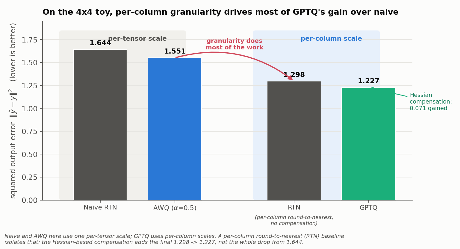
Read this comparison carefully, because it is easy to over-claim from it. The methods here do not share a granularity: naive and AWQ use one per-tensor scale, while GPTQ uses per-column scales. So the headline “GPTQ 1.227 < AWQ 1.551” mostly measures granularity, not algorithm. The per-column RTN row makes that explicit: simply switching to per-column scales, with no cleverness at all, already gets us to 1.298. GPTQ’s actual contribution, the Hessian-based error compensation, is the step from 1.298 to 1.227 - real, but a small slice of the total drop from 1.644 on this toy.

So the honest readings are:

• Granularity does most of the visible work here. Per-column scales stop the small columns from collapsing, which is where most of the naive error came from.
• The Hessian compensation adds a genuine but modest increment on top of per-column RTN. On this 4-value-per-column toy there is little room to redistribute; at real layer widths (thousands of channels) the compensation has far more room to work, which is why it matters more at scale.
• This is not a controlled AWQ-vs-GPTQ comparison. AWQ is shown at per-tensor and GPTQ at per-column; a fair face-off would fix bit-width, granularity, and calibration across both. There is no universal GPTQ-beats-AWQ (or vice versa) ranking across models, tasks, and settings, so treat the numbers as an illustration of mechanisms, not a benchmark.

---

3. AWQ vs. GPTQ: When to Use What

	AWQ	GPTQ
Core strategy	Scale salient channels up before quantization so they land more precisely on the grid	Round weights one at a time, compensate remaining weights using the Hessian
Mathematical tool	Per-channel activation magnitudes (\(\mathbf{s}_X\)) and a scalar $\alpha$	Inverse Hessian ($H^{-1} = (2 X X^T)^{-1}$), Cholesky-precomputed
Optimisation	Grid search over a single scalar $\alpha \in [0, 1]$	Closed-form column-by-column updates
Calibration needs	Only per-channel activation averages	Full Hessian computation: $O(d_{in}^2 \cdot n)$, plus Cholesky
Runtime per layer	Fast (no matrix inversions)	$O(d_{out} \cdot d_{in}^2)$
Overfitting risk	Lower, no per-weight reconstruction, just one scaling transform	Higher, reconstructs weights to fit calibration data
Serving path	W4A16: packed 4-bit weights + scales, fused dequant-GEMM kernel	W4A16: packed 4-bit weights + scales, fused dequant-GEMM kernel
Best for	Fast, hardware-friendly deployment	Maximum per-layer accuracy

A caution on that “Serving path” row, because the older framing (AWQ runs on standard kernels, GPTQ needs a custom one) is misleading. Both are weight-only W4A16: both serialize to packed low-bit weights plus scales, and both are served by a fused dequantize-then-GEMM kernel that reconstructs 16-bit weights before the matmul. Neither method’s quality mechanism (AWQ’s scaling, GPTQ’s compensation) runs at inference time at all - it is baked into the stored weights offline. Which serves faster depends on the exact serialized format and kernel, not on “AWQ vs GPTQ” as algorithms. Keep the three layers separate: algorithm (how weights are chosen), format (what lands on disk), kernel (what runs the matmul).

In practice:

• AWQ is a good fit when we want a simple, well-supported W4A16 path and minimal calibration machinery (just per-channel activation stats).
• GPTQ is a good fit when we can spend more offline compute on the Hessian and want the tightest per-layer reconstruction. Both are widely used and well-supported on model hubs; which wins on a given model, task, and bit-width is an empirical question, not a settled default, so it is worth measuring both rather than assuming one dominates.

Both methods are complementary to non-linear approaches: NF4 reshapes the grid to match the distribution, while AWQ and GPTQ keep the grid uniform but make the weights fit it better.

---

4. The Bigger Picture

Let’s zoom out and see where AWQ and GPTQ fit in the full landscape of quantization methods (covered across both articles in this series):

Method	Grid	Key idea	Cost	Best for
Linear Symmetric	Uniform	Equal-width bins	Instant	Baseline
Quantile	Non-uniform	Equal-count bins via percentiles	Sorting ($O(N \log N)$)	Theory
NF4	Non-uniform	Pre-computed quantile grid for normal distributions	Instant (lookup table)	QLoRA training
K-Means	Non-uniform	Data-adaptive clusters	Expensive (iterative)	Post-training compression
AWQ	Uniform	Activation-aware per-channel scaling	Fast (grid search)	Hardware-friendly inference
GPTQ	Uniform	Hessian-based error compensation across columns	Moderate ($O(d \cdot d^2)$)	High-accuracy inference

The core lesson across both articles: respecting the weight distribution is the key to preserving model quality at low bit-widths. Three strategies achieve this in different ways. Non-linear methods reshape the grid. AWQ protects the most sensitive channels. GPTQ compensates for rounding errors as it goes.

Underneath that lesson sits a sharper one. The naive view of quantization - just round every weight to the nearest INT4 value - misses three facts that every method in this series quietly exploits:

1. Weights interact with activations. The damage of a rounding error depends on what the weight gets multiplied by, not on its own magnitude.
2. Errors in different weights have different downstream impact. A handful of “salient” weights account for most of the output, and a much larger handful barely matter.
3. Errors can be redistributed. What one weight loses to rounding, another can partially absorb, if we know how the two are coupled.

AWQ handles points 1 and 2 with a clever pre-quantization scaling transform. GPTQ handles all three via iterative second-order compensation. Both push 4-bit quantization to surprisingly high quality, and they pave the way for even more aggressive schemes: 3-bit, 2-bit, and mixed-precision deployments where the same three principles are pushed even harder.

---

Appendix: Notation Reference

Symbol	Meaning
$W$	Original weight matrix, shape $d_{out} \times d_{in}$
$\hat W$ or $\hat W^{\text{method}}$	Quantized (and possibly compensated) weight matrix
$W’$	AWQ scaled weights: $W’ = W \cdot \text{diag}(\mathbf{s})$
$X$	Input activations on calibration data, shape $d_{in} \times n_{samples}$
\(\mathbf{s}_X\)	Per-channel average activation magnitude vector, shape $d_{in} \times 1$
$\mathbf{s}$	AWQ per-channel scaling vector, \(\mathbf{s} = \mathbf{s}_X^{\,\alpha}\), shape $d_{in} \times 1$
$\alpha$	AWQ scalar exponent controlling scaling aggressiveness, $\alpha \in [0, 1]$
$H$	Layer-wise Hessian, $H = 2 X X^T$, shape $d_{in} \times d_{in}$
$H^{-1}$	Inverse Hessian (precomputed via Cholesky)
\([H^{-1}]_{qq}\)	Diagonal entry at column $q$, the “stiffness” of that weight direction
\([H^{-1}]_{q, q+1:}\)	Row $q$ of $H^{-1}$ restricted to unquantized columns, the “spreading vector”
$\Delta$	Quantization step size (distance between adjacent grid points)
$\lambda$	GPTQ dampening constant, typically $0.01 \cdot \overline{\text{diag}(H)}$
$\text{quant}(w)$ or $Q(w)$	Nearest quantization grid point to $w$
$e_q$	Per-row quantization error in column $q$: $W_{:,q} - \hat W_{:,q}$
$B$	GPTQ block size (typically 128 for lazy batch updates)
$U$	Upper-triangular Cholesky factor of $H^{-1}$: $H^{-1} = U^T U$