Stats Primer: Parametric A/B Tests

Companion to Designing a Trustworthy A/B Test: the parametric (model-based) tests. Its sibling covers the non-parametric tests. Part of the inference arc, leading into sample size.

Designing a Trustworthy A/B Test set up the experiment; this post covers the parametric tests that analyze it, the ones that assume a distributional model (usually approximate normality, via the CLT). Building on the z and t tests from the previous post, we add ANOVA for three or more groups, the Chi-square test for categorical data, and the Bonferroni correction for multiple comparisons. The non-parametric alternatives are covered in the sibling post.

1. ANOVA

Analysis of Variance (ANOVA) is a statistical test used to determine if there are any statistically significant differences between the means of three or more independent groups. It essentially checks if the variation between the groups is larger than the variation within the groups.

The Concept Explained with an Example

Imagine a researcher wants to test if three different teaching methods (A, B, and C) have a different effect on student exam scores.

• Group A: Taught with Method A.
• Group B: Taught with Method B.
• Group C: Taught with Method C.

The researcher collects the final exam scores from students in each group.

The question ANOVA answers is: Are the differences in the average scores of these three groups large enough to conclude that the teaching methods have a real effect, or are the differences just due to random chance?

• Null Hypothesis ($H_0$): There is no difference between the teaching methods. The mean scores for all three groups are equal (${\mu_A = \mu_B = \mu_C}$).
• Alternative Hypothesis ($H_a$): At least one teaching method has a different mean score.

ANOVA works by comparing the variance between the groups’ average scores to the variance within each group’s individual scores. If the variance between the groups is significantly larger than the variance within the groups, we reject the null hypothesis.

The Mathematical Background

ANOVA’s math is centered around partitioning the total variation in the data into different components. This is done using “Sum of Squares.”

1. Partitioning the Variance (Sum of Squares)

• Sum of Squares Total (SST): Measures the total variation of every student’s score from the overall average score of all students combined. It represents the total variation in the data.
• Sum of Squares Between (SSB): Measures the variation of each group’s average score from the overall average score, i.e. the variation between the group means. (In a randomized experiment this between-group variation reflects the treatment effect; on observational data it is merely group-to-group variation and not automatically causal.)
• Sum of Squares Within (SSW): Measures the variation of each student’s score from their own group’s average. This represents the random, unexplained variation or “noise”.

The core relationship is: SST = SSB + SSW

2. Formulation Details

Here are the formulas for the Sum of Squares in a One-Way ANOVA (Analysis of Variance), broken down by component. To ensure clarity, let’s first define the notation used in the equations:

Notation Key

• $k$: Number of groups.
• $n$: Total number of observations (items) across all groups.
• $n_i$: The number of observations in the $i^{th}$ group.
• $x_{ij}$: The $j^{th}$ observation in the $i^{th}$ group.
• $\bar{x}_i$: The sample mean of the $i^{th}$ group.
• $\bar{x}$: The Grand Mean (the mean of all $n$ observations).

1. SST (Sum of Squares Total) This represents the total variation in the data. It compares every individual observation to the Grand Mean.

\[SST = \sum_{i=1}^{k} \sum_{j=1}^{n_i} (x_{ij} - \bar{x})^2\]

• Degrees of Freedom ($df_T$): $n - 1$

2. SSB (Sum of Squares Between) This represents the variation between the group means. It measures how much the groups differ from the Grand Mean (the “treatment” effect).

\[SSB = \sum_{i=1}^{k} n_i (\bar{x}_i - \bar{x})^2\]

• Degrees of Freedom ($df_B$): $k - 1$
• Note: If the sample sizes for all groups are equal, $n_i$ is a constant.

3. SSW (Sum of Squares Within) This represents the variation within each group. It measures the error or random variation (how far individual items are from their own group mean). This is often called $SSE$ (Sum of Squares Error).

\[SSW = \sum_{i=1}^{k} \sum_{j=1}^{n_i} (x_{ij} - \bar{x}_i)^2\]

Degrees of Freedom ($df_W$): $n - k$

3. Calculating Mean Squares

To get an average measure of variance (called a Mean Square), we divide the Sum of Squares by the degrees of freedom (df).

• Mean Square Between (MSB): This is the average variance between the groups.

  \[MSB = \frac{SSB}{k - 1}\]

  (where k is the number of groups)

• Mean Square Within (MSW): This is the average variance within the groups (the random noise).

  \[MSW = \frac{SSW}{N - k}\]

  (where N is the total number of students)

4. The F-statistic

The F-statistic is the final test statistic. It’s the ratio of the variance between the groups to the variance within the groups.

\[F = \frac{\text{Mean Square Between}}{\text{Mean Square Within}} = \frac{MSB}{MSW}\]

Interpretation:

• If the F-statistic is close to 1, it means the variation between the groups is about the same as the random variation within the groups, so there’s likely no treatment effect.
• If the F-statistic is large, it means the variation between the groups is much larger than the random variation, suggesting the treatment (the teaching method) has a real effect.

This calculated F-statistic is then compared to a critical value from an F-distribution to determine a p-value. If the p-value is below our significance level (e.g., 0.05), we reject the null hypothesis and conclude that at least one teaching method leads to a different average score.

Two clarifications on what ANOVA does and does not say. First, it tests whether the group means differ under the model’s assumptions (independent observations, roughly normal residuals, comparable group variances), not whether a treatment “caused” the difference absent a randomized design. Second, a significant global F-test tells us at least one group differs, but not which one(s). Identifying the specific pairs requires a post-hoc comparison (Tukey’s HSD, or pairwise tests with a multiplicity correction, the subject of the Bonferroni section below).

Range of the F-statistic

The F-statistic can take any value from 0 to positive infinity.

Since the F-statistic is a ratio of two variances (Mean Squares), which are always non-negative, the F-statistic itself can never be negative. There is no theoretical upper limit.

How to Find the Critical F-statistic

The critical F-statistic is the threshold value used to determine statistical significance. It’s the “line in the sand” on the F-distribution. If our experimental F-statistic exceeds this critical value, the result is significant.

We find this value using three key pieces of information:

1. Significance Level (α): The probability of a Type I error we’re willing to accept (commonly 0.05).
2. Numerator Degrees of Freedom (df₁): The degrees of freedom for the variance between groups. df₁ = k - 1, where k is the number of groups.
3. Denominator Degrees of Freedom (df₂): The degrees of freedom for the variance within groups. df₂ = N - k, where N is the total number of observations.

In practice, we use statistical software or an F-distribution table to find the critical value corresponding to these three parameters.

Example

Let’s use our previous example of testing three different teaching methods.

• Number of groups (k): 3
• Total students (N): Assume 10 students per group, so N = 30.
• Significance level (α): 0.05

1. Calculate the Degrees of Freedom:

• Numerator df₁ = k - 1 = 3 - 1 = 2
• Denominator df₂ = N - k = 30 - 3 = 27

2. Find the Critical Value:

• We need to find the critical F-value for an F-distribution with (2, 27) degrees of freedom at an alpha of 0.05.
• Using statistical software or an F-table, we find that the critical F-value is approximately 3.35.

Conclusion: This means if our experiment’s calculated F-statistic is greater than 3.35, the p-value will be less than 0.05, and we would reject the null hypothesis. We would conclude that at least one teaching method has a significantly different effect on student scores.

2. Chi-squared Test

The Chi-squared (${\chi^2}$) test is a statistical tool used to determine if there is a significant difference between what we expected to find and what we actually observed in a dataset.

Note: For a detailed analysis on Chi-squared distribution, please refer to the appendix.

There are two primary types:

• Test for Independence: Checks if two variables are related or independent of each other.
• Goodness of Fit Test: Checks if a single variable’s distribution matches what is expected.

Test for Independence

Step 1: State the Hypotheses

First, we state our null and alternative hypotheses. The null hypothesis always assumes that there is no relationship between the variables (e.g. snack choice and movie genre).

• Null Hypothesis ($H_0$): The two variables are independent. In our example, snack choice and movie genre are not related.
• Alternative Hypothesis ($H_a$): The two variables are dependent. Snack choice and movie genre are related.

Step 2: Create a Contingency Table

We organize our collected data into a table of observed frequencies.

Example Scenario: We survey 200 people at a movie theater to see if there’s a link between their favorite movie genre (Comedy, Action, Romance) and their preferred snack (Popcorn, Nachos).

Observed Data Table:

	Popcorn	Nachos	Row Total
Comedy	70	20	90
Action	45	25	70
Romance	25	15	40
Column Total	140	60	200

Step 3: Calculate Expected Frequencies

Next, we calculate what the frequencies would be in each cell if the null hypothesis were true (i.e., if the variables were perfectly independent).

The formula for each cell is: Expected Value = (Row Total × Column Total) / Grand Total

• Expected (Comedy, Popcorn): (90 × 140) / 200 = 63
• Expected (Comedy, Nachos): (90 × 60) / 200 = 27
• Expected (Action, Popcorn): (70 × 140) / 200 = 49
• And so on for every cell…

Step 4: Calculate the Chi-Squared Statistic

This step measures the difference between our observed data and our expected data.

The formula is:

\[{\chi^2 = \sum \frac{(O-E)^2}{E}}\]

Where:

• O = Observed frequency
• E = Expected frequency

We calculate this value for each cell and sum them up. The expected counts (row total × column total / grand total) are:

	Popcorn	Nachos
Comedy	63	27
Action	49	21
Romance	28	12

Summing $(O-E)^2/E$ over all six cells:

\[\chi^2 = \frac{(70-63)^2}{63} + \frac{(20-27)^2}{27} + \frac{(45-49)^2}{49} + \frac{(25-21)^2}{21} + \frac{(25-28)^2}{28} + \frac{(15-12)^2}{12} \approx 4.75.\]

Step 5: Make a Conclusion

Finally, we compare our calculated Chi-squared value to a critical value from a Chi-squared distribution table. This requires a significance level (usually α = 0.05) and the degrees of freedom.

• Degrees of Freedom = (Number of Rows - 1) × (Number of Columns - 1) = (3 - 1) × (2 - 1) = 2
• The critical Chi-squared value for 2 degrees of freedom at α = 0.05 is 5.99.

Conclusion:

• Since our calculated value (4.75) is less than the critical value (5.99), we fail to reject the null hypothesis.
• This means there is not enough statistical evidence to conclude that a relationship exists between movie genre preference and snack choice.

A validity note: the chi-square approximation relies on reasonably large expected counts (a common rule of thumb is every expected cell $\geq 5$, which holds here). For sparse tables with small expected counts, use Fisher’s exact test instead.

Goodness of Fit

The Chi-squared Goodness of Fit test determines if the observed frequency distribution of a single categorical variable matches a claimed or expected distribution. In essence, it tests how “well” our sample data “fits” a pre-existing theory.

Here is a step-by-step guide with an example.

The Scenario: M&M Colors

Let’s say the M&M company claims the following color distribution for their plain candies:

• Blue: 24%
• Green: 16%
• Orange: 20%
• Red: 13%
• Yellow: 14%
• Brown: 13%

We buy a large bag containing 400 M&Ms and want to test if our bag’s color distribution matches the company’s claim.

Step 1: State the Hypotheses

• Null Hypothesis ($H_0$): The color distribution of M&Ms in our bag is the same as the distribution claimed by the company.
• Alternative Hypothesis ($H_a$): The color distribution is different from the company’s claim.

Step 2: Organize Observed and Expected Frequencies

First, we count the M&Ms of each color in our bag (Observed). Then, we calculate how many of each color we would expect to see in a bag of 400 if the company’s claim is true.

Expected Count = Total Sample Size × Claimed Percentage For example, Expected Blue = 400 × 0.24 = 96.

Color	Observed (O)	Expected (E)
Blue	90	96
Green	70	64
Orange	82	80
Red	48	52
Yellow	55	56
Brown	55	52
Total	400	400

Step 3: Calculate the Chi-Squared Statistic

This step measures the total difference between our observed and expected counts.

The formula is:

\[{\chi^2 = \sum \frac{(O-E)^2}{E}}\]

We calculate this for each color and add them up:

• Blue: ${(90 - 96)^2 / 96 = 0.375}$
• Green: ${(70 - 64)^2 / 64 = 0.563}$
• Orange: ${(82 - 80)^2 / 80 = 0.050}$
• Red: ${(48 - 52)^2 / 52 = 0.308}$
• Yellow: ${(55 - 56)^2 / 56 = 0.018}$
• Brown: ${(55 - 52)^2 / 52 = 0.173}$

Total Chi-Squared Value (${\chi^2}$) = 0.375 + 0.563 + 0.050 + 0.308 + 0.018 + 0.173 = 1.487

Step 4: Make a Conclusion

Finally, we compare our calculated ${\chi^2}$ value to a critical value from a Chi-squared distribution table.

• Degrees of Freedom (df) = Number of Categories - 1 = 6 - 1 = 5
• For a significance level of α = 0.05 and df = 5, the critical value is 11.07.

Conclusion:

• Since our calculated ${\chi^2}$ value of 1.487 is much less than the critical value of 11.07, we fail to reject the null hypothesis.
• This means there is no statistically significant difference between the color distribution in our bag and the distribution claimed by the M&M company. Our sample data “fits” the expected distribution well.

Fundamental Differences with z and t-tests

The fundamental difference is the type of data they analyze: z-tests and t-tests are used for continuous data to compare means or proportions, while Chi-squared tests are used for categorical data to compare observed frequencies against expected frequencies.

This table summarizes the core distinctions between the tests.

Feature	Z-test / T-test	Chi-squared Test
Type of Data	Continuous (e.g., height, revenue, time) or Proportions	Categorical (e.g., colors, genres, yes/no)
Purpose	To compare the means or proportions of one or two groups.	To compare observed counts against expected counts.
Hypothesis About	A population parameter like the mean (${\mu}$) or proportion (${p}$).	A distribution (Goodness of Fit) or the relationship between two variables (Independence).

Scenarios for Usage

Here are practical scenarios where we would choose one test over the other.

When to Use a Z-test or T-test

We use these tests when the question is about averages or percentages.

• A/B Testing Conversion Rates: Comparing the conversion rate (a proportion) of two different website layouts to see which is more effective.
• Medical Research: Testing if a new drug lowers blood pressure more than a placebo by comparing the average blood pressure in the two groups of patients.
• Quality Control: A factory wants to know if the average weight of a product from the assembly line is equal to the target weight of 500g.
• Finance: Determining if the average daily return of a stock is significantly different from zero.

When to Use a Chi-squared Test

We use this test when the question is about counts, frequencies, or relationships between categories.

• Market Research: Determining if there is a relationship between a customer’s age group (18-25, 26-40, 41+) and their preferred social media platform (Instagram, Facebook, TikTok). This is a Test for Independence.
• Genetics: Testing if the observed counts of offspring with different traits (e.g., purple vs. white flowers) match the expected ratio predicted by Mendelian genetics. This is a Goodness of Fit Test.
• Polling Analysis: Analyzing survey results to see if voting preference (Party A, Party B, Undecided) is independent of the voter’s geographical region (North, South, East, West). This is a Test for Independence.
• Manufacturing: A company claims its bags of candy contain an equal number of red, green, and blue pieces. We count the pieces in a random sample to see if the observed frequencies match the expected frequencies. This is a Goodness of Fit Test.

3. Bonferroni’s Correction

The Bonferroni correction is a method used to counteract the increased risk of making a Type I error (a false positive) when we run multiple simultaneous hypothesis tests. It works by making the significance threshold for each individual test much stricter.

The Problem: Multiple Comparisons Inflate Error Rates

When we run a single A/B test with a significance level (alpha) of 0.05, we accept a 5% chance of finding a significant result when there isn’t one. However, when we run multiple tests at once, the probability of getting at least one false positive across the entire “family” of tests increases dramatically.

• 1 Test: The probability of a false positive is 5%.
• 3 Tests: The probability of at least one false positive increases to about 14%.
• 10 Tests: The probability of at least one false positive jumps to about 40%.

The Bonferroni correction is a simple, if conservative, way to control this Family-Wise Error Rate (FWER).

How the Bonferroni Correction Works

The method is straightforward: we divide our original alpha level by the number of tests we are performing.

\[\text{Corrected Alpha} = \frac{\text{Original Alpha}}{\text{Number of Tests } (n)}\]

This new, lower alpha becomes the p-value threshold we must beat for any individual test to be considered statistically significant.

Example: A/B/C/D Test on a Homepage

Imagine we want to test three new headlines (B, C, and D) against our current headline (A, the control) to see which one increases the sign-up rate.

This involves running three separate comparisons:

1. A vs. B
2. A vs. C
3. A vs. D

Our original significance level is $\alpha = 0.05$, and the number of tests is $n = 3$.

Without Correction (The Wrong Way)

We run the tests and get the following p-values:

• A vs. B: $p = 0.04$
• A vs. C: $p = 0.21$
• A vs. D: $p = 0.45$

Without correction, we would look at the A vs. B result ($p=0.04$) and, seeing it’s less than 0.05, declare headline B the winner.

With Bonferroni Correction (The Right Way)

We first calculate our new, stricter significance threshold:

\[\text{Corrected Alpha} = 0.05 / 3 \approx 0.0167\]

Now, we compare our p-values to this new threshold:

• A vs. B: $p = 0.04$ (This is greater than 0.0167) $\rightarrow$ Not Significant
• A vs. C: $p = 0.21$ (This is greater than 0.0167) $\rightarrow$ Not Significant
• A vs. D: $p = 0.45$ (This is greater than 0.0167) $\rightarrow$ Not Significant

Conclusion

After applying the Bonferroni correction, headline B’s $p = 0.04$ no longer clears the stricter bar. This does not prove B has no effect; it means that once we account for having run three comparisons, this result is not strong enough to act on. The correction guards against being routinely fooled by the most extreme of several noisy comparisons, rather than labeling any single result a definite false positive.

The Math Behind the Exploding Error Rate

The math behind the exploding chance of false positives relies on the basic rules of compound probability. The easiest way to see this is to calculate the probability of the opposite event: making zero false positives, and then subtracting that from 1.

Let’s assume:

• Significance level ($\alpha$) = 0.05 (a 5% chance of a false positive on any single test).
• Probability of NOT getting a false positive on a single test = $1 - 0.05 = 0.95$.

The Math with Examples

1 Test:

• The probability of getting at least one false positive is simply 0.05 (or 5%).

2 Tests: The probability of having no false positive on the first test AND no false positive on the second test is: $0.95 \times 0.95 = 0.95^2 = 0.9025$

• So, the probability of having at least one false positive is the complement: $1 - 0.9025 = 0.0975 \text{ (or 9.75%)}$

5 Tests: The probability of having no false positives across all five tests is: $0.95^5 \approx 0.774$

• The probability of having at least one false positive is: $1 - 0.774 = 0.226 \text{ (or 22.6%)}$

20 Tests: The probability of having no false positives across all twenty tests is: $0.95^{20} \approx 0.358$

• The probability of having at least one false positive is: $1 - 0.358 = 0.642 \text{ (or 64.2%)}$

As we can see, after just 20 tests, it’s more likely than not that we’ve been fooled by random chance at least once.

The General Formula

This demonstrates the formula for the Family-Wise Error Rate (FWER), which is the probability of making at least one Type I error across $n$ tests:

\[FWER = 1 - (1 - \alpha)^n\]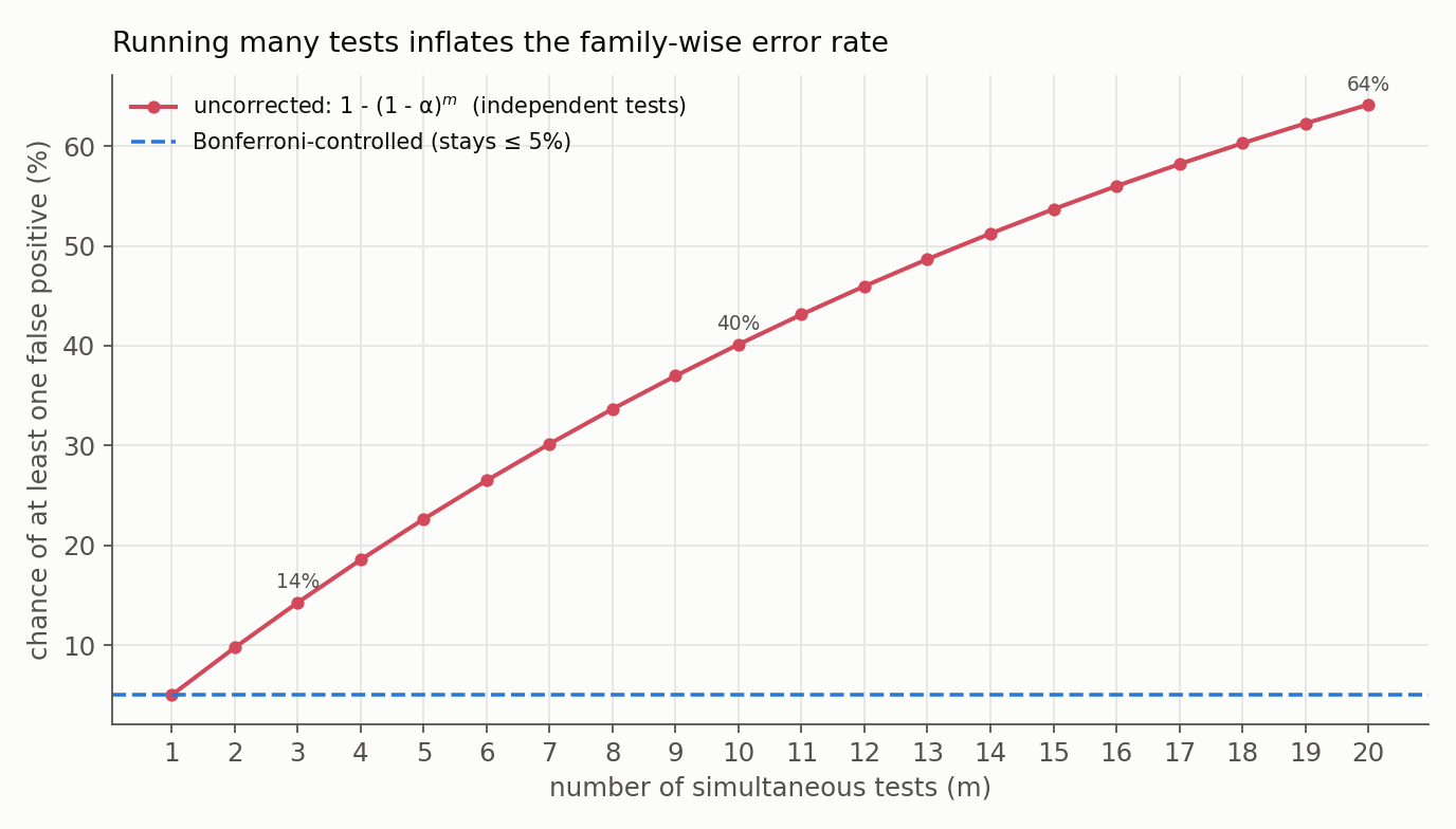

Two caveats keep this honest. First, the clean formula $1 - (1-\alpha)^n$ assumes the tests are independent; correlated metrics inflate the rate differently (usually less), so read it as an illustrative curve, not an exact figure for real dashboards. Second, and importantly, the Bonferroni correction itself does not require independence: it controls the family-wise error rate for any dependence structure, which is why it is so widely used (and why it is conservative). In practice: define the family of hypotheses up front, pick one primary metric, keep guardrails separate, and report adjusted p-values or simultaneous intervals. Bonferroni is the simplest correction; Holm’s step-down procedure is uniformly more powerful at the same guarantee, and Dunnett’s test is purpose-built for the common case of several variants compared against a single shared control.

Appendix

A. Demystifying the Chi-Squared Distribution

While ANOVA and Chi-Squared tests are practically executed with a few lines of code, understanding the math behind them provides a much stronger grasp of what our A/B test results actually mean. Here is a deep dive into the Chi-Squared ($\chi^2$) distribution.

1. Major Problem Areas Addressed by Chi-Squared

The Chi-Squared distribution isn’t just for comparing variations in A/B tests. It is a workhorse in statistics, primarily used when dealing with categorical data or variances. Its major applications include:

• Test of Independence: Determining if two categorical variables are related. (e.g., Does a user’s device type affect whether they click the ‘Buy’ button in our A/B test?)
• Goodness of Fit: Evaluating if a sample of categorical data matches an expected population distribution. (e.g., Is the traffic distributed evenly across our 4 test variants, or is our randomization flawed?)
• Test of Homogeneity: Assessing if different populations share the same distribution for a single categorical variable.
• Confidence Intervals for Variance: Estimating the population variance ($\sigma^2$) for normally distributed data.

2. The Chi-Squared Distribution: Definition and Properties

To understand the Chi-Squared distribution, we have to look back at the Standard Normal Distribution ($\mathcal{N}(0,1)$).

Definition: If we take a set of $k$ independent, standard normal random variables $Z_1, Z_2, \dots, Z_k$, square each of them, and sum them up, the resulting statistic follows a Chi-Squared distribution with $k$ degrees of freedom.

Mathematically, if $Z \sim \mathcal{N}(0,1)$, then:

\[Q = \sum_{i=1}^{k} Z_i^2 \sim \chi^2(k)\]

Key Properties:

• PDF (Probability Density Function): The exact shape of the distribution is defined by its degrees of freedom ($k$). For $x > 0$, the PDF is:

\[f(x; k) = \frac{x^{(k/2)-1} e^{-x/2}}{2^{k/2} \Gamma(k/2)}\]

(Where $\Gamma$ represents the Gamma function).

• Mean: The expected value is simply the degrees of freedom: $\mathbb{E}[Q] = k$.
• Variance: The variance grows with the degrees of freedom: $\text{Var}(Q) = 2k$.
• Geometric Interpretation: Because it is a sum of squares, the Chi-Squared distribution only exists for positive numbers (right-skewed). When $k$ is small (like 1 or 2), the bulk of the area is clustered near zero with a heavy right tail. As $k$ increases, the distribution shifts to the right and becomes more symmetric, eventually approximating a normal distribution (thanks to the Central Limit Theorem!).

3. Derivation of mean and variance

The Setup

Let $Q$ be a Chi-squared random variable with $k$ degrees of freedom. By definition, $Q$ is the sum of $k$ independent, squared standard normal variables:

\[Q = \sum_{i=1}^{k} Z_i^2\]

Where each $Z_i \sim \mathcal{N}(0, 1)$. Because they are standard normal, we know two facts about every $Z_i$:

1. Mean: $\mathbb{E}[Z_i] = 0$
2. Variance: $\text{Var}(Z_i) = 1$

1. Deriving the Mean: $\mathbb{E}[Q] = k$

We want to find the expected value of $Q$:

\[\mathbb{E}[Q] = \mathbb{E}\left[ \sum_{i=1}^{k} Z_i^2 \right]\]

Because of the linearity of expectation (the expected value of a sum is the sum of the expected values), we can bring the expectation inside the summation:

\[\mathbb{E}[Q] = \sum_{i=1}^{k} \mathbb{E}[Z_i^2]\]

Now, we need to find $\mathbb{E}[Z_i^2]$. We can find this using the standard variance formula: $\text{Var}(X) = \mathbb{E}[X^2] - (\mathbb{E}[X])^2$. Rearranging this for $Z_i$:

\[\mathbb{E}[Z_i^2] = \text{Var}(Z_i) + (\mathbb{E}[Z_i])^2\]

Plugging in our known values for a standard normal variable ($\text{Var} = 1$, Mean $= 0$):

\[\mathbb{E}[Z_i^2] = 1 + 0^2 = 1\]

Now substitute this back into our summation:

\[\mathbb{E}[Q] = \sum_{i=1}^{k} 1 = \underbrace{1 + 1 + \dots + 1}_{k \text{ times}} = k\]

2. Deriving the Variance: $\text{Var}(Q) = 2k$

We want to find the variance of $Q$:

\[\text{Var}(Q) = \text{Var}\left( \sum_{i=1}^{k} Z_i^2 \right)\]

Because the $Z_i$ variables are completely independent, the variance of their sum is simply the sum of their variances:

\[\text{Var}(Q) = \sum_{i=1}^{k} \text{Var}(Z_i^2)\]

To find $\text{Var}(Z_i^2)$, we use the variance formula again:

\[\text{Var}(Z_i^2) = \mathbb{E}[(Z_i^2)^2] - (\mathbb{E}[Z_i^2])^2\] \[\text{Var}(Z_i^2) = \mathbb{E}[Z_i^4] - (\mathbb{E}[Z_i^2])^2\]

We already know from the previous step that $\mathbb{E}[Z_i^2] = 1$. To find $\mathbb{E}[Z_i^4]$, we look at the moments of the standard normal distribution. A known property of the standard normal distribution $\mathcal{N}(0, \sigma^2)$ is that its fourth moment is $3\sigma^4$. Since $\sigma = 1$, $\mathbb{E}[Z_i^4] = 3(1)^4 = 3$.

Substitute these back into the variance equation for a single $Z_i^2$:

\[\text{Var}(Z_i^2) = 3 - (1)^2 = 2\]

Finally, substitute this back into our summation for $Q$:

\[\text{Var}(Q) = \sum_{i=1}^{k} 2 = \underbrace{2 + 2 + \dots + 2}_{k \text{ times}} = 2k\]

4. Where Does the Formula $\sum \frac{(O-E)^2}{E}$ Come From?

When we run a Chi-Squared test, we use Pearson’s cumulative test statistic:

\[\chi^2 = \sum \frac{(O_i - E_i)^2}{E_i}\]

But how does a formula about Observed ($O$) and Expected ($E$) counts connect to the sum of squared normal variables? Here is the step-by-step intuition:

Step 1: The Standard Normal Variable Recall the formula to standardize a normal variable (the z-score):

\[Z = \frac{X - \mu}{\sigma}\]

If we square this, we get a Chi-Squared distribution with 1 degree of freedom:

\[Z^2 = \frac{(X - \mu)^2}{\sigma^2}\]

Step 2: Connecting to Counts In categorical data (like counting clicks vs. non-clicks), our expected count $E$ acts as the mean ($\mu$). A fascinating property of counting processes (which often follow a Poisson distribution) is that the variance is approximately equal to the mean.

Therefore, if the mean $\mu \approx E$, then the variance $\sigma^2 \approx E$.

Step 3: Substituting the Terms If we take our squared z-score formula and substitute $X$ with our Observed count ($O$), $\mu$ with our Expected count ($E$), and $\sigma^2$ with $E$, we get:

\[Z^2 \approx \frac{(O - E)^2}{E}\]

Step 4: Summing the Categories An A/B test has multiple categories or cells (e.g., Variant A Clicks, Variant A No-Clicks, Variant B Clicks, Variant B No-Clicks). Since the total test statistic is the sum of these independent standard normal squares, we sum them across all $k$ categories:

\[\chi^2 = \sum_{i=1}^{k} \frac{(O_i - E_i)^2}{E_i}\]

The Intuition: We square the difference $(O - E)$ so that negative and positive errors don’t cancel each other out. We divide by $E$ to standardize the error. Missing the expected count by 10 is a massive deal if we only expected 5 clicks, but it’s statistically meaningless if we expected 10,000 clicks. Dividing by $E$ scales the “surprise” factor perfectly.

B. The Strange Similarity between Chi-Squared Test and Test with KL-Divergence to measure Goodness of Fit

The Goodness of Fit test could just as well have been executed via KL-Divergence, and spotting that connection is a sharp catch. The chi-square goodness-of-fit test and KL divergence are closely related. In fact, the chi-square test can be viewed as a second-order approximation to KL divergence. They come from the same conceptual framework: measuring the discrepancy between two probability distributions. (A word of caution on terminology: KL is a divergence, not a distance metric. It is asymmetric, $D_{KL}(\hat p \Vert p) \neq D_{KL}(p \Vert \hat p)$, and does not obey the triangle inequality, so “distance” is loose language throughout this section.)

Let’s unpack that.

1. What the Chi-Square Goodness-of-Fit Test Measures

Suppose:

• Observed counts: ($O_i$)
• Expected counts: ($E_i = n p_i$)

The chi-square statistic is $\chi^2 = \sum_i \frac{(O_i - E_i)^2}{E_i}$

If we convert counts to empirical probabilities: $\hat{p}_i = \frac{O_i}{n}$, then $E_i = n p_i$.

Substitute into the statistic:

\[\chi^2 = n \sum_i \frac{(\hat{p}_i - p_i)^2}{p_i}\]

So chi-square is essentially a weighted squared distance between distributions.

2. KL Divergence Between Distributions

KL divergence between the empirical distribution ($\hat{p}$) and the hypothesized distribution ($p$) is:

\[D_{KL}(\hat{p} \| p) = \sum_i \hat{p}_i \log \frac{\hat{p}_i}{p_i}\]

This measures how different the two distributions are.

3. The Mathematical Connection

If the empirical probabilities are close to the true ones: $\hat{p}_i \approx p_i$, we can do a Taylor expansion of the log term.

3.1: Define the delta

We define a small deviation: $\delta_i = \hat p_i - p_i$. Then $\hat p_i = p_i + \delta_i$.

3.2: Rewrite the Ratio

The log term becomes:

\[\log\left(\frac{\hat p_i}{p_i}\right) = \log\left(\frac{p_i + \delta_i}{p_i}\right) = \log\left(1 + \frac{\delta_i}{p_i}\right)\]

So KL divergence becomes

\[D_{KL} = \sum_i(p_i + \delta_i) \log \left(1 + \frac{\delta_i}{p_i}\right)\]

3.3: Use Taylor Expansion of log(1+x)

For small $x$:

\[\log(1+x) = x - \frac{x^2}{2} + \frac{x^3}{3} - ...\]

If $x$ is small we keep the first two terms:

\[\log(1+x) \approx x - \frac{x^2}{2}\]

So,

\[\log\left(1 + \frac{\delta_i}{p_i}\right) \approx \frac{\delta_i}{p_i} - \frac{1}{2}\frac{\delta_i^2}{p_i^2}\]

3.4: Substitute Back Into KL

Now plug this approximation into

\[D_{KL} = \sum_i (p_i + \delta_i) \log\left(1 + \frac{\delta_i}{p_i}\right)\]

So,

\[D_{KL} \approx \sum_i (p_i + \delta_i) \left(\frac{\delta_i}{p_i} - \frac{1}{2}\frac{\delta_i^2}{p_i^2}\right) = \sum_i\left(\delta_i + \frac{1}{2}\frac{\delta_i^2}{p_i} - \frac{1}{2}\frac{\delta_i^3}{p_i^2}\right)\]

3.5: Drop Small Higher-Order Terms

Because deviations are small: $\delta_i^3 \approx 0$.

Also notice: $\sum_i \delta_i = 0$, because both distributions sum to 1. So the ($\delta_i$) term vanishes.

What remains:

\[D_{KL} \approx \frac{1}{2}\sum_i\frac{\delta_i^2}{p_i}\]

3.6: Replace $\delta_i$ and Convert Back to Counts

Recall: $\delta_i = \hat p_i - p_i$

So,

\[D_{KL} \approx \frac{1}{2}\sum_i\frac{(\hat p_i - p_i)^2}{p_i}\]

Empirical probability: $\hat p_i = \frac{O_i}{n}$. Expected probability: $p_i = \frac{E_i}{n}$.

Plugging in gives

\[2nD_{KL} \approx \sum_i \frac{(O_i - E_i)^2}{E_i}\]

which is exactly the chi-square statistic.

4. What This Means Conceptually

Both tests measure how far the empirical distribution is from the hypothesized distribution.

But they do it differently:

Method	Distance Type
Chi-square	quadratic approximation
KL divergence	information-theoretic

So, $\chi^2 \approx 2n D_{KL}$ for small deviations.

5. Deeper Statistical Connection

The likelihood ratio test for multinomial distributions uses:

\[G = 2 \sum_i O_i \log\frac{O_i}{E_i}\]

This is called the G-test. It can be written as:

\[G = 2n D_{KL}(\hat{p} \| p)\]

So the G-test is literally KL divergence scaled by sample size.

Interestingly Chi-square test and G-test (KL-based) are asymptotically equivalent: both converge to a chi-square distribution under the null. They are distinct statistics that agree in large samples, not interchangeable finite-sample formulas, and they can differ noticeably when counts are small.

Why do They Look So Similar?

Because both arise from the same deeper object: divergence between distributions. In fact they are both part of the broader class of f-divergences.

6. Closing Thoughts

A nice way to think about it:

• KL divergence is the information-theoretic divergence (asymmetric, not a metric).
• Chi-square is the quadratic approximation to it, used for easier analysis.

Historically chi-square came first because it was easier to compute before computers.

One Elegant Way to Remember It:

Three related goodness-of-fit statistics:

Statistic	Formula	Interpretation
Pearson $\chi^2$	($\sum (O-E)^2/E$)	quadratic error
G-test	($2\sum O\log(O/E)$)	KL divergence
Likelihood ratio	same as G-test	information loss

For large samples they give nearly the same result.

---

Continue to sample size for A/B tests, or revisit experiment design.

Resources

• NIST/SEMATECH e-Handbook: Chi-Square Goodness-of-Fit Test and One-Way ANOVA.
• Wasserstein, R. L. & Lazar, N. A. (2016). The ASA Statement on p-Values: Context, Process, and Purpose. The American Statistician, 70(2), 129-133.