Linear Thompson Sampling: Exploring by Sampling Plausible Reward Lines

The contextual-bandits post worked one LinUCB decision with every matrix on the page, then replayed the same decision with Linear Thompson Sampling in a few paragraphs. That replay showed what Linear TS does (sample a plausible line per arm, play the best one) but skipped nearly everything that makes it usable: why the belief is Gaussian, how a draw is actually produced, how often each arm gets chosen, how it relates to LinUCB, and how to tune it. This post fills those gaps on the same running example, with the same numbers.

The last of those questions hides the most interesting result. Re-running the previous post’s simulation across a sweep of tuning values shows that Linear TS’s weaker score there came almost entirely from a cold-start trap - a prior centred in the wrong place - and not from the sampling idea itself.

---

1. The Running Example, Recapped

A content site chooses between two article formats, short-form and deep-dive, for each visitor. Before choosing it sees one context number, a session-intent score $z \in [-1, 1]$, and each arm’s expected engagement is a line in $z$ (unknown to the learner):

\[\mu_{\text{short}}(z) = 0.55 - 0.20\,z, \qquad \mu_{\text{deep}}(z) = 0.55 + 0.20\,z, \qquad r = \mu_a(z) + \mathcal{N}(0, 0.1^2)\]

The context vector is $x = (1, z)^\top$, so each arm owns an intercept and a slope, $\theta_a = (\theta_{a,0}, \theta_{a,1})^\top$. After 12 rounds (six per arm), the previous post’s ridge bookkeeping with $\lambda = 1$ stood at:

\[A_{\text{s}} = \begin{bmatrix} 7 & -0.70\\ -0.70 & 2.99 \end{bmatrix}, \quad \hat{\theta}_{\text{s}} = \begin{bmatrix} 0.472\\ -0.155 \end{bmatrix}, \qquad A_{\text{d}} = \begin{bmatrix} 7 & -1.90\\ -1.90 & 2.51 \end{bmatrix}, \quad \hat{\theta}_{\text{d}} = \begin{bmatrix} 0.446\\ 0.049 \end{bmatrix}\]

All six deep-dive observations sit at $z \le 0.3$, so its slope is poorly pinned down. A new visitor arrives at $z^\ast = 0.6$. LinUCB scored the arms 0.936 (short-form) and 1.200 (deep-dive) and served the deep-dive, on the strength of its large uncertainty bonus out at high intent. We now make the same decision the Bayesian way.

---

2. From Beta to Gaussian: The Same Idea, One Level Up

The first bandit post ran Thompson Sampling on click-through rates: each ad had a Beta belief, each round drew one plausible rate per ad, and the largest draw won. Linear TS keeps every step and swaps the object of belief from a number to a line:

	Beta-Bernoulli Thompson Sampling	Linear Thompson Sampling
Unknown per arm	One click rate $\mu_a$	One line $\theta_a$ (intercept, slope)
Belief	$\text{Beta}(\alpha_a, \beta_a)$	$\mathcal{N}(\hat{\theta}_a,\; v^2 A_a^{-1})$
Starting point	$\text{Beta}(1, 1)$: every rate equally plausible	$\mathcal{N}(0,\; v^2 I / \lambda)$: lines near zero
Update after reward $r$	$\alpha_a \mathrel{+}= r$, $\beta_a \mathrel{+}= 1 - r$	$A_a \mathrel{+}= x x^\top$, $b_a \mathrel{+}= r\,x$
One draw is	A plausible click rate	A plausible reward line
Decision	Play the largest draw	Play the largest $x^\top \tilde{\theta}_a$
Uncertainty shrinks with	Pulls of the arm	Pulls in this direction of context

The update row is the surprising one: Linear TS’s Bayesian update is exactly LinUCB’s bookkeeping. Here is why.

Why the update is the same bookkeeping

Assume Gaussian noise of scale $\sigma$ and a Gaussian prior $\theta \sim \mathcal{N}(0, \tau^2 I)$. Gaussian beliefs are easiest to update in their precision form (precision is inverse covariance): every observation $(x, r)$ adds its information, much as each click adds one to a Beta count:

\[\Sigma_{\text{new}}^{-1} = \Sigma_{\text{old}}^{-1} + \frac{x x^\top}{\sigma^2}, \qquad \Sigma_{\text{new}}^{-1} \mu_{\text{new}} = \Sigma_{\text{old}}^{-1} \mu_{\text{old}} + \frac{r\, x}{\sigma^2}\]

Multiply both equations by $\sigma^2$ and name the results $A = \sigma^2 \Sigma^{-1}$ and $b = \sigma^2 \Sigma^{-1} \mu$: they become $A \mathrel{+}= x x^\top$ and $b \mathrel{+}= r\,x$, starting from $A = (\sigma^2/\tau^2)\, I = \lambda I$ and $b = 0$. So after any history,

\[\theta_a \mid \mathcal{D} \;\sim\; \mathcal{N}\!\left(A_a^{-1} b_a,\; \sigma^2 A_a^{-1}\right) = \mathcal{N}\!\left(\hat{\theta}_a,\; \sigma^2 A_a^{-1}\right)\]

The posterior mean is the ridge estimate, the ridge penalty is the prior ($\lambda = \sigma^2 / \tau^2$), and the matrix that sized LinUCB’s bonus is the posterior covariance up to $\sigma^2$. This is conjugacy, Beta-Bernoulli’s Gaussian sibling, and it is exact under the stated assumptions (the appendix of the previous post derives the same result in batch form). The ridge stabilizer was never an ad-hoc fix; it is a prior belief that the line sits near zero.

Hold on to that last phrase: near zero. With $\lambda = 1$ and the sampling scale below, the prior puts each arm’s baseline engagement at $0 \pm 0.15$ (one standard deviation), while real engagement runs around 0.55. Section 6 shows what that costs.

The sampling scale v

Implementations sample from $\mathcal{N}(\hat{\theta}_a, v^2 A_a^{-1})$, with a tunable $v$ in the slot the theorem gives to $\sigma$. We use $v = 0.15$ against a true noise of $\sigma = 0.10$, so the cloud we sample is a deliberately inflated, posterior-shaped exploration distribution rather than the exact posterior. Inflation is the safe direction: $\sigma$ is unknown in practice, and a belief that is too tight stops exploring too early. The regret analysis of Agrawal and Goyal (2013) inflates far more, to $v = R\sqrt{(24/\epsilon)\, d \ln(1/\delta)}$ for $R$-sub-Gaussian noise. Abeille and Lazaric (2017) explain why: the proof needs each draw to be optimistic with a fixed probability, and guaranteeing that in $d$ dimensions costs an extra $\sqrt{d}$ factor of regret compared with LinUCB. Practitioners typically run far smaller values than the theory licenses.

What the belief looks like

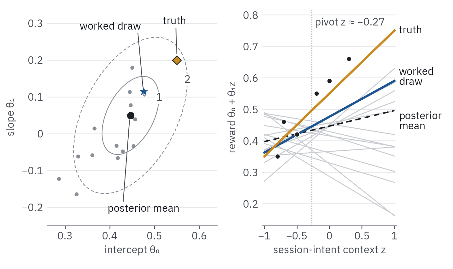Figure 1. Each point in the deep-dive’s belief is one line on the right. We draw fourteen (intercept, slope) pairs from the inflated cloud with $v = 0.15$ and plot each one twice: as a point, with ellipses at one and two standard units, and as a reward line. A higher intercept comes with a higher slope, so the lines pivot near the observations instead of drifting up and down together.

The left panel is the belief itself: every point is a candidate (intercept, slope) pair, and the ellipses mark one and two standard units of the inflated cloud. The right panel is the same cloud read as lines. Three features of the figure carry the intuition:

• The cloud is tilted. The deep-dive’s correlation between intercept and slope is $+0.45$. Its data sits on the left, so every plausible line must pass close to the observations near $z \approx -0.3$; a line raised at $z = 0$ must therefore be steeper to stay anchored there.
• The lines pivot where the data is. The fan is narrowest at $z \approx -0.27$, exactly where LinUCB’s bonus curve from the previous post is smallest ($x^\top A_{\text{d}}^{-1} x = 0.180 + 0.272z + 0.501z^2$, minimized at $z = -0.27$). Same matrix, same geometry.
• The truth is inside the cloud, though off its centre. The true $(0.55, 0.20)$ sits 1.8 standard units from the mean: an honest belief, centred wrong because of six noisy, lopsided points and ridge shrinkage, but wide enough to admit the truth. Sampling is how the bandit finds out.

---

3. How a Draw Is Actually Made

Sampling a correlated Gaussian reduces to sampling independent standard normals and reshaping them. Factor the covariance as $A_a^{-1} = L L^\top$ with $L$ lower-triangular (the Cholesky factor), draw $u \sim \mathcal{N}(0, I)$, and set

\[\tilde{\theta}_a = \hat{\theta}_a + v\, L\, u, \qquad \text{Cov}(v L u) = v^2 L\, \text{Cov}(u)\, L^\top = v^2 A_a^{-1}\]

For the deep-dive arm:

\[A_{\text{d}}^{-1} = \begin{bmatrix} 0.180 & 0.136\\ 0.136 & 0.501 \end{bmatrix} = L L^\top, \qquad L = \begin{bmatrix} 0.424 & 0\\ 0.321 & 0.631 \end{bmatrix}, \qquad vL = \begin{bmatrix} 0.0636 & 0\\ 0.0481 & 0.0947 \end{bmatrix}\]

The previous post’s draw used $u = (0.468, 0.445)$:

\[\tilde{\theta}_{\text{d}} = \begin{bmatrix} 0.446\\ 0.049 \end{bmatrix} + \begin{bmatrix} 0.0636 \cdot 0.468\\ 0.0481 \cdot 0.468 + 0.0947 \cdot 0.445 \end{bmatrix} = \begin{bmatrix} 0.476\\ 0.114 \end{bmatrix}\]

The factor reads like a recipe. The first normal, $u_1$, moves the intercept and drags the slope along with it (the 0.0481 entry): that is the tilt from the figure. The second, $u_2$, adjusts only the slope. And $\lVert u \rVert = 0.65$, well inside the typical range for a two-dimensional standard normal: an ordinary draw, not a lucky outlier. The short-form arm’s draw $(0.466, -0.142)$ came from $u = (-0.099, 0.159)$, almost exactly its mean.

In production we never form $A_a^{-1}$. We take the Cholesky factor of $A_a$ itself, $A_a = R R^\top$, and solve the triangular system $R^\top w = u$; then $\text{Cov}(w) = R^{-\top} R^{-1} = A_a^{-1}$, and $\tilde{\theta}_a = \hat{\theta}_a + v\,w$. Factorizing costs $O(d^3)$ for $d$ features, and rank-one Cholesky updates bring the per-round cost down to $O(d^2)$ when $d$ runs into the hundreds.

---

4. The Decision, Replayed, and Its Exact Probability

With both draws in hand, the decision is the one we saw before:

1. Score the visitor on each sampled line: $x^{\ast\top} \tilde{\theta}_{\text{s}} = 0.466 - 0.142 \cdot 0.6 = 0.381$ and $x^{\ast\top} \tilde{\theta}_{\text{d}} = 0.476 + 0.114 \cdot 0.6 = \mathbf{0.545}$.
2. Play the larger: the deep-dive.
3. Update the deep-dive’s $A_{\text{d}}, b_{\text{d}}$ with the observed reward, exactly as LinUCB would.

But one draw is one outcome of a random process. Rerun the same round and the short-form might win. The useful question is: how often does Linear TS serve each arm to this visitor?

The answer needs no simulation. A score $x^\top \tilde{\theta}_a$ is a fixed linear combination of a Gaussian vector, so it is a one-dimensional Gaussian:

\[x^\top \tilde{\theta}_a \;\sim\; \mathcal{N}\!\left(x^\top \hat{\theta}_a,\; v^2\, x^\top A_a^{-1} x\right)\]

Its mean is the arm’s predicted reward, and its standard deviation is $v$ times the same uncertainty width LinUCB uses. At $z^\ast = 0.6$ the widths were 0.557 and 0.724, so

\[S_{\text{s}} \sim \mathcal{N}(0.379,\; 0.0836^2), \qquad S_{\text{d}} \sim \mathcal{N}(0.476,\; 0.1085^2)\]

The two draws are independent, so their difference is Gaussian too, with mean $0.476 - 0.379 = 0.097$ and standard deviation $\sqrt{0.0836^2 + 0.1085^2} = 0.137$:

\[P(\text{deep-dive}) = P(S_{\text{d}} - S_{\text{s}} > 0) = \Phi\!\left(\frac{0.097}{0.137}\right) = \Phi(0.71) = 0.76\]

Linear TS serves the deep-dive to 76% of visitors in this exact situation, and the short-form to the other 24%. LinUCB serves the deep-dive to all of them. A Monte Carlo check with 200,000 paired draws gives 0.760, and the implementation in section 8 reproduces it.

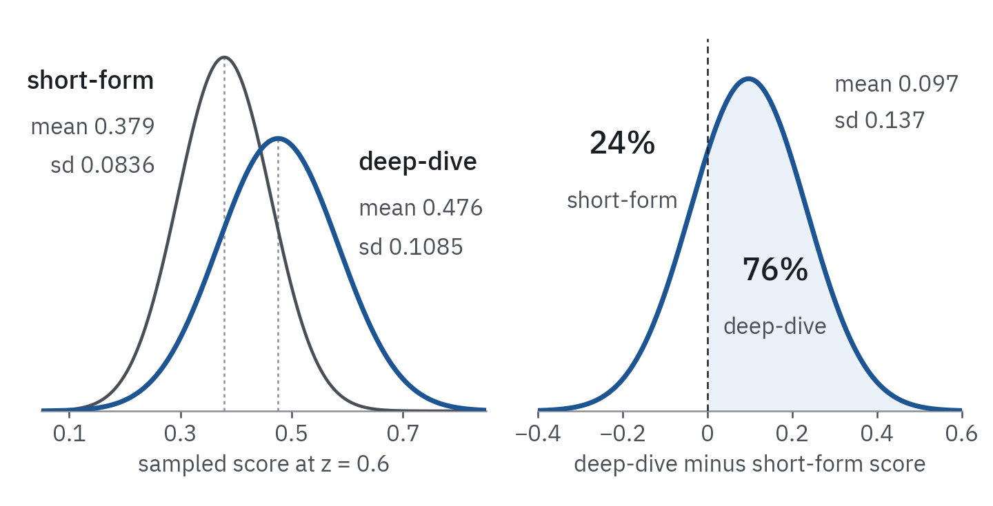Figure 2. The propensity is one Gaussian area. At $z^\ast = 0.6$ each arm’s sampled score is a one-dimensional Gaussian whose spread is $v$ times LinUCB’s width. We subtract one from the other, and the share of the difference above zero is the probability that Linear TS serves the deep-dive: 76%, with no simulation needed.

This 0.76 is the propensity that the previous post’s logging section asks us to record for offline evaluation. Notice that it must be computed: the realized draw (deep-dive wins, 0.545 vs 0.381) says nothing about it. With two arms the closed form above is exact. With $K$ independent arms the probability that arm $k$ wins is a one-dimensional integral, $\int \phi_k(s) \prod_{j \ne k} \Phi_j(s)\, ds$, cheap to evaluate numerically. Monte Carlo over the per-arm score distributions covers everything else.

---

5. LinUCB With a Random Multiplier

Put the two score formulas side by side. A one-dimensional Gaussian is its mean plus its standard deviation times a standard normal, so in distribution:

\[\text{LinUCB:}\quad p_a(x) = x^\top \hat{\theta}_a + \alpha \sqrt{x^\top A_a^{-1} x}\] \[\text{Linear TS:}\quad x^\top \tilde{\theta}_a = x^\top \hat{\theta}_a + v\, Z_a \sqrt{x^\top A_a^{-1} x}, \qquad Z_a \sim \mathcal{N}(0, 1) \text{ fresh for each arm and round}\]

Linear TS is LinUCB whose fixed multiplier $\alpha$ has been replaced by a random one, $v Z_a$. Both read their uncertainty from the same matrix; they differ only in what they multiply it by. (The identity holds arm by arm for a single context. When one draw $\tilde{\theta}_a$ scores many contexts at once, as on a page of candidates, those scores share a draw and are correlated, which the per-context view ignores.)

In the worked round, the deep-dive’s draw corresponded to $Z_{\text{d}} = (0.545 - 0.476)/0.1085 = 0.64$ and the short-form’s to $Z_{\text{s}} = 0.02$. The effective multipliers were $v Z = 0.096$ and $0.003$, against LinUCB’s $\alpha = 1$ for both. Three consequences follow from the identity:

1. No optimism on average. $\mathbb{E}[v Z_a] = 0$, so each arm’s expected score is just its prediction. Uncertainty does not raise the score; it raises the spread of the score, and with it the arm’s chance of producing the top draw.
2. The boundary stays where the evidence puts it. Linear TS serves each arm half the time exactly where the fitted lines cross. Uncertainty only decides how gradually the probability changes on either side.
3. Exploration never fully switches off. Wherever both arms keep some uncertainty, both keep some probability.

Sweeping the visitor’s $z$ across the whole range, with the state frozen after 12 rounds, makes all three visible:

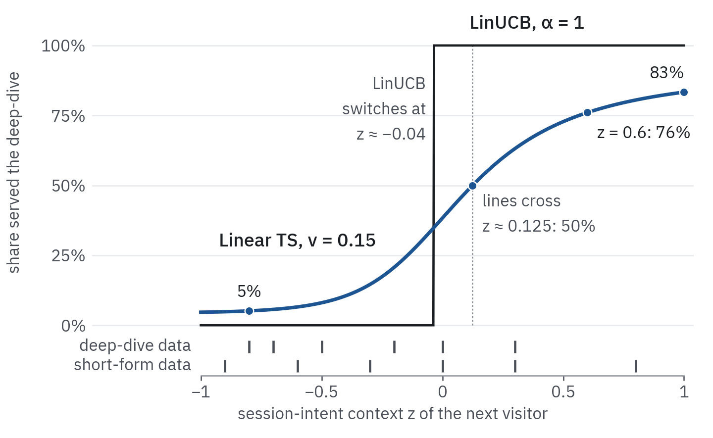Figure 3. Same state after 12 rounds: LinUCB’s hard switch and Linear TS’s soft one. We freeze both policies’ state and sweep the next visitor’s $z$. LinUCB with $\alpha = 1$ jumps from never to always serving the deep-dive, while Linear TS with $v = 0.15$ moves smoothly through 50% where the fitted lines cross; even at $z = 1$ it still sends 17% of visitors to the short-form, so its exploration never fully stops.

LinUCB switches at $z \approx -0.04$, before the fitted lines cross at $z \approx 0.125$: the deep-dive’s larger bonus pulls the switch left, so optimism hands the uncertain arm extra territory, deterministically. Linear TS keeps its 50% point at the crossing and hedges around it: 21% deep-dive at $z = -0.2$, 69% at $z = 0.4$, 83% at $z = 1$. Even at $z = -0.8$, where the evidence is clearly against it, the deep-dive gets 5% of visitors.

That last number can look wasteful. It is the price of a belief that admits being wrong. At $z = 1$, the region the deep-dive has never seen, it is really worth 0.75 against the short-form’s 0.35, yet the current belief can only give it 83%. Data will sharpen both tails, and the probabilities move toward 0 and 1 as the widths shrink. Linear TS keeps exploring for as long as the uncertainty lasts.

---

6. Choosing v, and the Cold-Start Trap

The previous post’s simulation (2,500 rounds, 200 seeded runs) gave LinUCB with $\alpha = 1$ a median contextual pseudo-regret of about 2.9 and Linear TS with $v = 0.15$ about 8.8, with a 90th percentile near 32. Its footnote called that gap “a property of the tuning pair, not a theorem”. Here is the tuning, swept. The environment and policies are the same as before, but every run draws fresh seeds, so at $v = 0.15$ the sweep lands at a median of 8 with a 90th percentile of 47: the median barely moves, while a tail that rests on the worst 20 of 200 runs shifts with the seeds. $v$ ranges from 0.025 to 1.0, and a second series moves the prior’s intercept from 0 to 0.5:

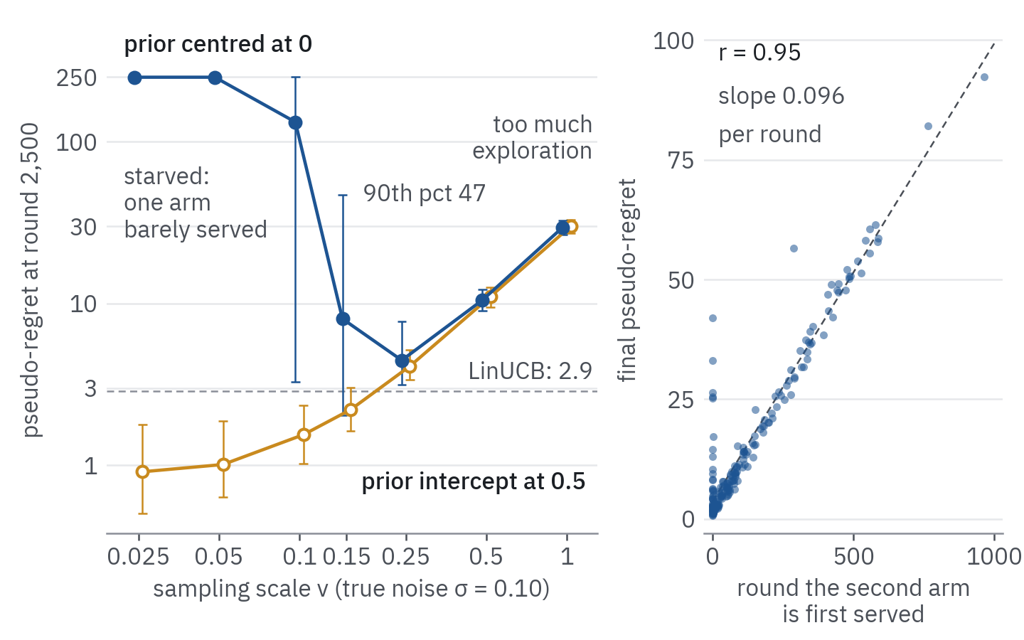Figure 4. With the prior at zero, the wait for the second arm is the regret. Left: we run 200 seeded simulations of 2,500 rounds for each value of $v$ and plot the median with bars from the 10th to the 90th percentile; the curve with filled markers keeps the prior at zero as in the previous post, and the curve with open markers centres the prior intercept at 0.5. Right: for $v = 0.15$ with the zero prior, each dot is one run, and the round at which it first serves the second arm predicts its final regret (r = 0.95).

The filled-marker curve, with the prior centred at zero as in the previous post, has two failure modes:

• Too much exploration (right side). At $v = 0.5$ and $v = 1$ the cloud is so wide that Linear TS keeps serving the wrong arm long after the lines are learned. Regret is still climbing at round 2,500, and both priors agree, because data has long since overwhelmed them.
• Starvation (left side). At $v \le 0.05$, regret sits at about 250, as bad as the context-blind bandit from the previous post. At $v = 0.05$, 98.5% of runs serve one of the arms at most three times in 2,500 rounds.

The starvation mechanism is pure cold start. In round 1 both arms have identical beliefs and one wins a coin flip. It earns around 0.55, and within a handful of serves its intercept estimate climbs toward 0.5. The untried arm’s belief is still the prior: a line near zero whose sampled score at the visitor has standard deviation $v\sqrt{1 + z^2}$. To be served at all, that draw must beat roughly 0.5. With $v = 0.05$ that takes a draw seven to ten standard deviations above its mean, so it effectively never happens. With $v = 0.15$ it takes about three, which happens eventually.

That “eventually” is Linear TS’s regret at $v = 0.15$. The right panel plots, for each of the 200 runs, the round at which the second arm is first served against the run’s final regret. The median wait is 54 rounds, 10% of runs wait more than 412, and the slowest waits 965. The correlation with final regret is 0.95, and the fitted slope is 0.096 per round of waiting: essentially the context-blind leak rate $\mathbb{E}[0.20 \lvert z \rvert] = 0.10$ from the previous post, because a policy serving one arm to everyone is a context-blind policy. The long tail that worried us there (a 90th percentile near 32 against a median of 8.8) is simply the slow-starting runs. A 1,000-seed rerun of the zero-prior $v = 0.15$ case gives a median of 8.6 and a 90th percentile of 38, consistent with the previous post’s 8.8 and 32.

LinUCB with $\alpha = 1$ escapes only because an untried arm’s bonus, $\alpha \sqrt{1 + z^2} \ge 1$, outbids the served arm’s prediction plus its shrinking bonus. The trap belongs to the prior, not the algorithm: LinUCB with $\alpha \le 0.25$ starves in exactly the same way, at about 250.

Centre the prior and the picture changes. Setting the prior intercept to 0.5 (initialize $b_a = \lambda\, m$ with $m = (0.5, 0)$, or equivalently subtract a 0.5 baseline from every reward) removes the trap. The open-marker curve then falls steadily as $v$ shrinks: 2.2 at $v = 0.15$, 1.0 at $v = 0.05$, now below LinUCB’s 2.9. Centring rescues small values of $\alpha$ too: LinUCB reaches a median of 0.9 at $\alpha = 0.25$, where the zero prior starved it. Under a fair comparison the two families finish close together, and the previous post’s gap was mostly a cold-start artifact.

One more honesty check: with the prior centred, even $v = 0$, pure greedy play on the posterior mean, scores about 1.0 here. Our toy is unusually kind to greedy. Visitors arrive uniformly on both sides of the crossover, so whichever arm is served collects well-spread contexts and its line gets pinned down for free. Bastani, Bayati, and Khosravi (2021) prove that greedy is rate-optimal for two arms under exactly this kind of covariate diversity. Deliberate exploration earns its keep when contexts are narrow or clustered, when there are many features, or when the reward changes over time. That is the normal production case, and it is not this toy.

What carries over into practice:

• Centre the prior. Set the prior mean to a sensible baseline, such as the historical average reward, or subtract that baseline from rewards. A prior mean of zero only makes sense when zero is a plausible reward.
• Start $v$ near the noise scale. Estimate $\sigma$ from residuals, then inflate modestly (one to two times). If $\sigma$ is unknown or drifts, a Normal-inverse-gamma prior learns it from the data instead.
• Judge the tail, not the median. Starvation shows up first in the upper percentiles across seeds. One lucky run can hide it entirely.
• Tune on logs when possible. Offline policy evaluation over logged propensities (section 4) scores candidate values of $v$ without deploying them.

---

7. Where Randomization Pays: Batches, Delays, and Logging

Section 6 showed that, with good tuning, Linear TS and LinUCB use the same uncertainty and finish close together. The practical case for Linear TS rests on what the randomness does in production.

Batched and delayed updates. Real systems rarely update after every reward: models refresh every few minutes or hours, and rewards arrive late (the production post worked through a six-hour cadence). Between refreshes, LinUCB applies a frozen deterministic rule, so every visitor in a region of context space gets the same arm until the next refresh, whether that arm is right or not. Linear TS samples fresh for every decision, so it spreads traffic across the plausible lines within the batch. Chapelle and Li (2011) measured this in a non-contextual simulation of news recommendation. As feedback moved from every step to every 1,000 steps, UCB’s regret grew more than ninefold (24,145 to 226,220) while Thompson Sampling’s grew about six-and-a-half-fold (9,105 to 59,256), staying below UCB’s at every delay.

Propensities are built in. Offline evaluation needs each action’s logged probability. LinUCB’s are 0 or 1, so it needs an explicit exploration floor before any counterfactual question can be answered. Linear TS assigns every eligible arm a probability that is usually strictly between 0 and 1 (section 4’s 0.76 and 0.24). Logging still requires computing it, and when an arm’s probability drops toward zero, IPS weights explode just as they do with a thin floor.

Priors carry knowledge. A model trained offline, or the posterior from last month, can become today’s prior by initializing $A_a$ and $b_a$ from it: the Gaussian belief is a natural container for “what we already know”.

Drift needs forgetting. Like LinUCB, Linear TS’s belief only ever tightens. If rewards drift, multiply $A_a$ and $b_a$ by a factor slightly below one at each refresh, so that old evidence fades and the cloud can widen again.

---

8. Implementation

The whole algorithm fits in a small class: Cholesky-based sampling of $A_a$ (no explicit inverse), LinUCB’s update, and the propensity calculation from section 4.

import numpy as np
from scipy.linalg import cho_factor, cho_solve, solve_triangular
from scipy.stats import norm


class LinearThompson:
    """Disjoint Linear Thompson Sampling: one Gaussian belief per arm."""

    def __init__(self, n_arms, d, lam=1.0, v=0.15, prior_mean=None, seed=0):
        self.v = v
        self.rng = np.random.default_rng(seed)
        m = np.zeros(d) if prior_mean is None else np.asarray(prior_mean, float)
        self.A = np.array([lam * np.eye(d) for _ in range(n_arms)])  # precision (up to v^2)
        self.b = np.array([lam * m for _ in range(n_arms)])          # lam * m centres the prior

    def _mean(self, a):
        return cho_solve(cho_factor(self.A[a], lower=True), self.b[a])    # theta_hat = A^{-1} b

    def sample_theta(self, a):
        R = np.linalg.cholesky(self.A[a])                     # A = R R^T, R lower-triangular
        u = self.rng.standard_normal(len(self.b[a]))
        w = solve_triangular(R.T, u, lower=False)             # Cov(w) = A^{-1}, no inverse formed
        return self._mean(a) + self.v * w

    def select(self, x):
        scores = [x @ self.sample_theta(a) for a in range(len(self.A))]
        return int(np.argmax(scores))

    def update(self, a, x, r):
        self.A[a] += np.outer(x, x)                           # same bookkeeping as LinUCB
        self.b[a] += r * x

    def choice_probs(self, x, n_mc=100_000):
        """Propensity of each arm at context x, from the per-arm score distributions."""
        means = np.array([x @ self._mean(a) for a in range(len(self.A))])
        sds = np.array([self.v * np.sqrt(x @ np.linalg.solve(self.A[a], x)) for a in range(len(self.A))])
        if len(means) == 2:                                   # closed form: P(score_1 > score_0)
            p1 = norm.cdf((means[1] - means[0]) / np.hypot(*sds))
            return np.array([1 - p1, p1])
        draws = self.rng.normal(means, sds, size=(n_mc, len(means)))
        return np.bincount(draws.argmax(1), minlength=len(means)) / n_mc


# Rebuild the 12-round state from the contextual-bandits post and query z* = 0.6.
history = {0: ([-0.9, -0.6, -0.3, 0.0, 0.3, 0.8], [0.78, 0.61, 0.65, 0.50, 0.45, 0.42]),   # short-form
           1: ([-0.8, -0.7, -0.5, -0.2, 0.0, 0.3], [0.35, 0.46, 0.42, 0.55, 0.59, 0.66])}  # deep-dive
bandit = LinearThompson(n_arms=2, d=2)
for arm, (zs, rs) in history.items():
    for z, r in zip(zs, rs):
        bandit.update(arm, np.array([1.0, z]), r)

x_star = np.array([1.0, 0.6])
print("posterior means:", [bandit._mean(a).round(3) for a in (0, 1)])
print("P(short), P(deep):", bandit.choice_probs(x_star).round(3))
picks = [bandit.select(x_star) for _ in range(20_000)]
print("empirical share of deep-dive over 20,000 draws:", np.mean(picks).round(3))

Running it reproduces the hand-worked numbers:

posterior means: [array([ 0.472, -0.154]), array([0.446, 0.049])]
P(short), P(deep): [0.24 0.76]
empirical share of deep-dive over 20,000 draws: 0.761

(The short-form slope prints as $-0.154$ rather than $-0.155$: the unrounded value is $-0.1545$.) To centre the prior as section 6 recommends, pass prior_mean=[0.5, 0.0].

---

9. LinUCB vs. Linear Thompson Sampling, Side by Side

Question	LinUCB	Linear Thompson Sampling
Uncertainty	Confidence ellipsoid around $\hat{\theta}_a$	Posterior distribution over $\theta_a$
Exploration	Fixed multiplier: $\alpha \sqrt{x^\top A_a^{-1} x}$	Random multiplier: $v Z_a \sqrt{x^\top A_a^{-1} x}$
Same history, same next action?	Always	No: each arm has a choice probability
Decision boundary	Hard switch, shifted toward the more uncertain arm	Soft, with its 50% point where the fitted lines cross
Propensity for offline evaluation	0 or 1: needs an exploration floor	Computable: closed form for two arms, a 1-D integral or Monte Carlo beyond
Batched or delayed updates	Frozen deterministic rule between refreshes	Randomizes within each batch
Prior knowledge	Less direct (initialize $A_a, b_a$)	Natural: it is a prior
Main tuning	Exploration coefficient $\alpha$	Sampling scale $v$, plus the prior mean
Cold-start failure	Small $\alpha$ with a zero-centred prior	Small $v$ with a zero-centred prior

---

Where This Leaves Us (and the Epilogue Ahead)

Linear TS turned out to be less exotic than its reputation. Its update is LinUCB’s bookkeeping, its uncertainty is LinUCB’s width, and its decision is LinUCB’s score with a random multiplier. What the randomness buys is a choice probability: a soft decision boundary, exploration that fades only as fast as the evidence warrants, propensities ready for offline evaluation, and robustness when updates arrive in batches. What it demands is a prior in the right place, a lesson that applies to LinUCB just as much.

One assumption ran through both contextual posts: a continuous reward modelled by a linear function with Gaussian noise. Clicks and purchases are binary, and for those the line must pass through a link function. Linear TS then has a logistic cousin: Chapelle and Li’s experiments used a Laplace-approximated Gaussian posterior over logistic-regression weights, sampled from just as we sample here. That link function is the doorway to the next article, the epilogue on generalized linear models, which closes the series.

---

Resources

• Agrawal and Goyal (2013), Thompson Sampling for Contextual Bandits with Linear Payoffs - the Linear TS algorithm and its regret analysis, with the inflated sampling scale.
• Abeille and Lazaric (2017), Linear Thompson Sampling Revisited - why the analysis needs inflation, and the $\sqrt{d}$ price of it.
• Chapelle and Li (2011), An Empirical Evaluation of Thompson Sampling - Thompson Sampling’s empirical case, including delayed feedback and a Laplace-approximated logistic variant.
• Russo, Van Roy, Kazerouni, Osband, and Wen (2018), A Tutorial on Thompson Sampling - a broad, readable treatment of Thompson Sampling beyond the linear case.
• Bastani, Bayati, and Khosravi (2021), Mostly Exploration-Free Algorithms for Contextual Bandits - when greedy play is enough, and the covariate-diversity condition behind it.