Stats Primer: How to Choose the Right Sample Size for Your A/B Tests
We’re almost at the end of our journey of A/B Testing. There are few concepts we need to understand before wrapping up. So, here we go.
1. Pre-requisites: The Statistical Foundation
Before diving into the math, we must understand the “rules of the game” regarding errors and sample sizes.
Type I and Type II Errors (The Boy Who Cried Wolf)
In hypothesis testing, we risk making two types of mistakes. Let’s use the fable of “The Boy Who Cried Wolf” to understand them.
- Type I Error ($\alpha$ - False Positive):
- The Scenario: The boy cries “Wolf!” when there is actually no wolf and villagers come.
- Technical Meaning:
- Null Hypothesis ($H_0$): “There is no wolf!” $\rightarrow$ which is true.
- We (villagers) falsely reject the null Hypothesis ($H_0$). So, it’s a false positive error.
- In A/B Testing: You conclude that Version B is better than Version A, when in reality, there is no difference. This is determined by your Significance Level ($\alpha$), typically set to 0.05, accepting a 5% chance of a false positive.
- Type II Error ($\beta$ - False Negative):
- The Scenario: The boy cries “Wolf!”. The wolf actually appears, but the villagers don’t come.
- Technical Meaning:
- Null Hypothesis ($H_0$): “There is no wolf!” $\rightarrow$ which is false.
- We (villagers) mistakenly fail to reject the null Hypothesis ($H_0$). So, it’s a false negative error.
- In A/B Testing: Version B is actually better, but your test fails to detect it.
Statistical Power
Statistical power is the probability that your experiment will correctly detect a real difference if one exists (Power = $1 - \beta$).
- A test with high power is like a strong magnifying glass, sensitive enough to spot genuine improvements.
- The industry standard is 80%, meaning you accept a 20% chance of missing a real winner (Type II error).
The Link to Sample Size
To avoid these errors, you cannot simply stop a test when you see a win. You must calculate a sample size before starting. The sample size is the number of users required to satisfy your chosen $\alpha$ (risk of false positive) and Power (ability to avoid false negative).
2. Sample Size Calculation for various A/B Tests
1-Sample Z-Test
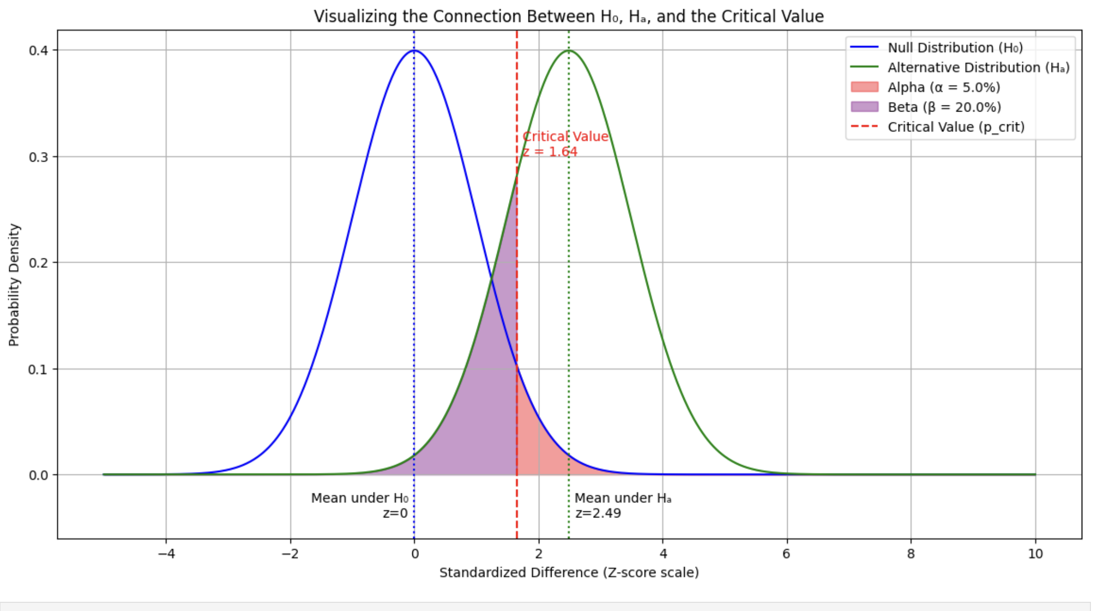
Formulation: The critical value is defined from the perspective of the null hypothesis ($H_0$) and the alternative hypothesis ($H_a$).
\[\text{Critical Value} = \mu_0 + Z_{\alpha/2} \cdot \frac{\sigma}{\sqrt{n}}\] \[\text{Critical Value} = \mu_a - Z_{\beta} \cdot \frac{\sigma}{\sqrt{n}}\]Min Sample Size Derivation: To find $n$, we set the two critical value expressions equal to each other:
\[\mu_0 + Z_{\alpha/2} \frac{\sigma}{\sqrt{n}} = (\mu_0 + \delta) - Z_{\beta} \frac{\sigma}{\sqrt{n}}\]Rearranging to isolate $n$:
\[\frac{\sigma}{\sqrt{n}}(Z_{\alpha/2} + Z_{\beta}) = \delta\] \[\sqrt{n} = \frac{\sigma(Z_{\alpha/2} + Z_{\beta})}{\delta}\] \[n = \frac{(Z_{\alpha/2} + Z_{\beta})^2 \sigma^2}{\delta^2}\]- (Where $\delta$ is the Minimum Detectable Effect)
2-Sample Z-Test
Min Sample Size Derivation: We use the standard error of the difference between two means ($SE = \sqrt{\frac{2\sigma^2}{n}}$).
\[Z_{\alpha/2} \cdot \sqrt{\frac{2\sigma^2}{n}} = \delta - Z_{\beta} \cdot \sqrt{\frac{2\sigma^2}{n}}\]Solving for $n$:
\[n = \frac{2(Z_{\alpha/2} + Z_{\beta})^2 \sigma^2}{\delta^2}\]Rationale for $SE = \sqrt{\frac{2\sigma^2}{n}}$
1. The General Rule (Variance Sum Law)
\[Var(\bar{x}_1 - \bar{x}_2) = Var(\bar{x}_1) + Var(\bar{x}_2)\]
When you subtract two independent random variables (like two sample means, $\bar{x}_1$ and $\bar{x}_2$), their variances add up. Even though you are calculating the difference in means ($\bar{x}_1 - \bar{x}_2$), the uncertainty (variance) from both groups accumulates.2. Variance of a Single Sample Mean
\[Var(\bar{x}) = \frac{\sigma^2}{n}\]
The variance of a single sample mean is the population variance divided by the sample size:So, substituting this into the general rule:
\[Var(\bar{x}_1 - \bar{x}_2) = \frac{\sigma_1^2}{n_1} + \frac{\sigma_2^2}{n_2}\]3. The Simplifying Assumptions
The specific formula $\frac{2\sigma^2}{n}$ is derived by applying two constraints commonly used in experimental design:Equal Variances: We assume the population variance for both groups is the same ($\sigma_1^2 = \sigma_2^2 = \sigma^2$).
Equal Sample Sizes: We assume we use the same sample size for both groups ($n_1 = n_2 = n$).4. The Final Derivation
\[Var(\bar{x}_1 - \bar{x}_2) = \frac{\sigma^2}{n} + \frac{\sigma^2}{n} = \frac{2\sigma^2}{n}\]
Substitute these assumptions back into the equation:
1-Proportion Z-Test
Formulation: The critical value is defined from the perspective of the null hypothesis ($H_0$) and the alternative hypothesis ($H_a$). We’re using a one-tailed test here.
\[p_{crit} = p_0 + Z_{\alpha} \sqrt{\frac{p_0(1-p_0)}{n}}\] \[p_{crit} = p_a - Z_{\beta} \sqrt{\frac{p_a(1-p_a)}{n}}\]Min Sample Size Derivation: Since both equations describe the same critical value point, we set them equal to each other
\[p_0 + Z_{\alpha} \sqrt{\frac{p_0(1-p_0)}{n}} = p_a - Z_{\beta} \sqrt{\frac{p_a(1-p_a)}{n}}\]Rearrange the terms to isolate $n$
\[Z_{\alpha} \sqrt{\frac{p_0(1-p_0)}{n}} + Z_{\beta} \sqrt{\frac{p_a(1-p_a)}{n}} = p_a - p_0\] \[n = \left( \frac{Z_{\alpha}\sqrt{p_0(1-p_0)} + Z_{\beta}\sqrt{p_a(1-p_a)}}{p_a - p_0} \right)^2\]
2-Proportion Z-Test
Formulation: The critical value is defined from the perspective of the null hypothesis ($H_0$) and the alternative hypothesis ($H_a$). We’re using a two-tailed test here.
\[d_{crit} = 0 + Z_{\alpha/2} \cdot SE\] \[d_{crit} = (p_1 - p_2) - Z_{\beta} \cdot SE\]Min Sample Size Derivation: We equate the critical values defined by $\alpha$ and $\beta$.
\[Z_{\alpha/2} \sqrt{\frac{p_1(1-p_1)}{n} + \frac{p_2(1-p_2)}{n}} = (p_1 - p_2) - Z_{\beta} \sqrt{\frac{p_1(1-p_1)}{n} + \frac{p_2(1-p_2)}{n}}\]Solving for $n$ gives the standard formula:
\[n = \frac{(Z_{\alpha/2} + Z_{\beta})^2 [p_1(1-p_1) + p_2(1-p_2)]}{(p_1 - p_2)^2}\]
Everything Else
For z-tests and t-tests, we have simple algebra formulas. For ANOVA, Chi-Square, and Simulation tests, the math becomes too complex for pen-and-paper algebra because it involves “non-central” probability distributions.
Here is how you determine the sample size ($n$) for these more complex scenarios.
ANOVA and Chi-Square (Parametric Tests)
Since there is no simple formula like $n = \frac{(z_{\alpha}+z_{\beta})^2 \sigma^2}{\delta^2}$, we use Power Analysis. You need to define four inputs to solve for the fifth (Sample Size).
The 4 Inputs You Must Define
- Significance Level ($\alpha$): Usually 0.05.
- Power ($1-\beta$): Usually 0.80 (80% chance of finding the effect if it exists).
- Degrees of Freedom (Groups): How many groups are you comparing? (A/B/C/D…)
- Effect Size: This is the hardest part. You must estimate “how wrong” the Null Hypothesis is.
| Test | Effect Size Metric | How to estimate it? |
|---|---|---|
| ANOVA (Continuous) | Cohen’s $f$ | $f = \sqrt{\frac{\eta^2}{1-\eta^2}}$ Rule of thumb: Small=0.1, Medium=0.25, Large=0.4 |
| Chi-Square (Counts) | Cohen’s $w$ (or Cramér’s V) | $w = \sqrt{\sum \frac{(P_{observed} - P_{expected})^2}{P_{expected}}}$ Rule of thumb: Small=0.1, Medium=0.3, Large=0.5 |
How to actually calculate it
Do not try to derive this manually. Use software.
- G*Power: The gold standard free tool for this. You literally select “F-test (ANOVA)” or “Chi-square”, input the effect size (0.25), alpha (0.05), and power (0.80), and it gives you $n$.
- Python/R:
- Python:
statsmodels.stats.power.FTestAnovaPower().solve_power(effect_size=0.25, alpha=0.05, power=0.8) - R:
pwr.anova.test(k=3, f=0.25, sig.level=0.05, power=0.8)
- Python:
Permutation & Bootstrap Tests (Simulation Methods)
This is trickier. Because these tests don’t assume a specific distribution (like the Normal or F-distribution), there is no formula to calculate sample size.
Instead, you must run a Simulation-Based Power Analysis. You essentially “fake” an experiment on your computer thousands of times to see what sample size works.
The Algorithm (How to do it step-by-step)
Step 1: Create a “Synthetic Truth”
Decide what effect you hope to find.- Example: “I suspect Group A has a mean of 10 and Group B has a mean of 12, with a standard deviation of 3.”
Step 2: Pick a starting $n$
Let’s guess you need $n=30$ per group.- Step 3: Run the “Outer Loop” (The Power Simulation)
- Generate random data for Group A ($n=30, \mu=10, \sigma=3$) and Group B ($n=30, \mu=12, \sigma=3$).
- Run your Permutation Test (or Bootstrap) on this fake data to get a p-value.
- Record: Did the p-value drop below 0.05? (1 = Yes, 0 = No).
- Repeat this 1,000 times.
- Step 4: Calculate Power If you rejected the Null 600 times out of 1,000, your Power is 60%.
- Goal: We want 80%.
- Step 5: Adjust and Repeat Since 60% < 80%, increase $n$ to 40 and repeat Step 3. Keep increasing $n$ until your rejection rate hits 80%.
The “Rule of Thumb” Shortcut If you don’t have time to write a simulation script, use the “Parametric + 15%” rule.
- Calculate the sample size required for a standard parametric test (e.g., t-test or ANOVA).
- Add 15% to that number.
- Non-parametric tests are generally less powerful than parametric ones (because they ignore distribution info), so they usually need slightly more data to find the same effect.
Summary Table
| Test Type | How to find Sample Size ($n$) |
|---|---|
| Z-test / T-test | Simple Algebra Formula |
| ANOVA / Chi-Square | Use G*Power or statsmodels (Effect Size inputs required) |
| Permutation / Bootstrap | Simulation Loop (Generate fake data $\to$ Check Power $\to$ Adjust $n$) |
3. What is Sample Ratio Mismatch (SRM)?
When we design an A/B test, we define a target traffic split: most commonly a 50/50 allocation between the Control and Treatment groups. Sample Ratio Mismatch (SRM) occurs when the actual, observed traffic split during the experiment deviates from this planned ratio by a statistically significant margin.
For example, if we plan a 50/50 split and run the test until we hit 100,000 total visitors, we expect roughly 50,000 in Control and 50,000 in Treatment. If our final counts are 50,500 in Control and 49,500 in Treatment, it might look like a minor 1% variance. However, at scale, we must prove whether this deviation is just random noise or a symptom of a broken experiment.
How to Detect SRM: The Chi-Square Test in Action
To prove that the mismatch isn’t just random noise, we don’t use a standard Z-test or t-test, we use a Chi-Square Goodness of Fit test. This test compares our observed counts ($O$) against our expected counts ($E$).
The test statistic is calculated as:
\[\chi^2 = \sum \frac{(O - E)^2}{E}\]Let’s plug in our example numbers of 100,000 total visitors:
- Expected ($E$): 50,000 Control, 50,000 Treatment
- Observed ($O$): 50,500 Control, 49,500 Treatment
Step 1: Calculate the Chi-Square value
- Control: $\frac{(50,500 - 50,000)^2}{50,000} = \frac{500^2}{50,000} = \frac{250,000}{50,000} = 5$
- Treatment: $\frac{(49,500 - 50,000)^2}{50,000} = \frac{(-500)^2}{50,000} = \frac{250,000}{50,000} = 5$
- Total $\chi^2$ $= 5 + 5 = \mathbf{10}$
Step 2: Compare against the Critical Value Because we have 2 categories (Control and Treatment), our Degrees of Freedom ($df$) is $2 - 1 = \mathbf{1}$.
Now we look at the Chi-Square distribution table for $df=1$:
- If we use a standard significance level of $\alpha = 0.05$ (95% confidence), the critical value is 3.84. Since $10 > 3.84$, we would flag this as a significant mismatch.
- However, industry standard for SRM is much stricter, typically set at $\alpha = 0.001$ (99.9% confidence). Why? Because a false positive on an SRM check forces us to throw away an entire experiment, so we want to be absolutely certain it’s broken. The critical value for $\alpha = 0.001$ is 10.83.
The Verdict: Because our calculated $\chi^2$ of 10 is just barely less than the strict critical value of 10.83 (yielding a p-value of roughly ~0.0015), we would technically fail to reject the null hypothesis at the 0.001 level. We can cautiously proceed with the experiment, but this is a massive warning sign. If the gap widened even slightly (e.g., 50,600 vs 49,400, resulting in $\chi^2 = 28.8$), it would trigger a massive SRM alert, and we would have to invalidate the test.
The Implications: Why SRM is a Nightmare
If a test triggers a true SRM, every other statistical calculation in our experiment is instantly invalidated. We cannot trust our Z-tests, our p-values, or our effect sizes.
Here is why SRM breaks the experiment:
- Violation of Randomization: A/B testing relies on the core assumption of a Randomized Controlled Trial (RCT): that the only difference between the two groups is the treatment itself. SRM indicates a systemic bias in how users are being sorted or tracked, meaning the groups are no longer mutually exclusive and unbiased.
- Simpson’s Paradox & Survivorship Bias: If our Treatment variant causes older, slower devices to crash before the tracking pixel fires, our Treatment group will artificially look like it has a higher conversion rate because the lowest-performing users were literally excluded from the data pool. The SRM is the only warning sign that this happened.
- False Positives/Negatives: Because the sample sizes ($N$) are skewed, the standard errors used in our Z-tests will be calculated incorrectly, drastically inflating our Type I or Type II error rates beyond our designed $\alpha$ and $\beta$ thresholds.
Common Engineering Culprits Behind SRM
In digital adtech and web experimentation, SRM is rarely a math error, it is almost always a telemetry or engineering bug. Common causes we see include:
- Redirect Latency: If the Treatment requires a heavy client-side redirect, users on slow connections might bounce before the redirect completes and the analytics event fires. Control gets logged, Treatment does not.
- Tracking Bugs in the Variant: The new code in the Treatment might inadvertently break the analytics tracking pixel for a specific browser or edge case.
- Bad Hash Functions: The randomizer assigning users to groups (usually via hashing a user ID or cookie) might not be uniformly distributed, causing collisions that favor one bucket.
- Bot Traffic Skew: Bots often do not manage cookies properly. If a bot gets assigned to Treatment, drops its cookie, and returns, it might get re-assigned, skewing our unique user counts.