Beyond A/B Testing: Running a Bandit in Production

Multi-Armed Bandits: Part 1: Thompson Sampling and UCB · Part 2: Running a Bandit in Production

Part 1 built the two workhorse bandit policies on one running example (three ad creatives, Ad A, Ad B, Ad C, with true click rates of 10%, 20%, and 35%), derived what regret measures, and raced the policies over 200 seeded simulations. Everything there lived inside the teaching model: stationary Bernoulli arms, one reward per round, observed immediately, and a simulator that knows the true rates. This post is about what happens when a bandit leaves that model: choosing between the two policies on engineering grounds, rewards that arrive days late, the clean inference adaptive allocation quietly destroys, and how to measure regret at all when nobody knows the best arm. It ends where the contextual-bandits post begins: one global winner is often the wrong question.

1. Conceptual Differences: UCB vs. Thompson Sampling

Same problem, two philosophies, different operational mechanics:

Consideration	How each algorithm behaves
Statistical Philosophy	UCB - frequentist: point estimates plus a concentration-based optimism bonus.
	TS - Bayesian: full posterior distributions, updated continuously.
Decision Rule	UCB - deterministic index (unless randomization is added explicitly): the same state yields the same next arm.
	TS - randomized probability matching: plays each arm in proportion to the probability it is optimal.
Prior Information	UCB - less direct: enters through initialization or model design (warm starts are possible, just not natural).
	TS - native: shape the prior (part 1, section 3.e) - but that also makes it vulnerable to prior and model misspecification.
Reproducibility	UCB: same state, same action - easy to replay and audit.
	TS: replaying a decision requires logging the model state and the random draw.
Delays and Batches	UCB: with a frozen state, a deterministic index can pour an entire batch into one arm; needs pending-count bookkeeping or a delay-aware variant.
	TS: keeps randomizing under a frozen posterior, which diversifies a batch - but is not delay-proof, and needs the same bookkeeping (section 2).

The practical reality: both algorithms carry rigorous regret guarantees under the teaching model, and both generalize beyond it - UCB to sub-Gaussian and other reward classes, TS to any likelihood with a tractable (or approximable) posterior. The choice is an engineering and modeling trade-off, not a leaderboard. TS asks us to trust a prior and a likelihood, and pays us back with natural randomization and evidence-handling; UCB asks only for bounded rewards, and pays us back with determinism and auditability. Teams valuing replayable decisions lean UCB-ward; teams with usable historical evidence and delayed feedback often lean TS-ward - and either lean should be revisited against the actual reward distribution, delays, and tuning.

---

2. When Rewards Arrive Late: The Delay Problem

Every loop in part 1 quietly assumed the same choreography: choose an arm, observe the reward, update, face the next visitor. That is roughly true when the reward is an immediate click; it is false for most business rewards. A checkout completes minutes after the impression, a sign-up converts hours after the ad, a trial becomes a paid subscription 14 days after the install. For the metrics companies actually care about, decision-to-feedback lag is the norm, not an edge case.

The scale is easy to underestimate. At 10 impressions per second with a 24-hour attribution window, early conversions may trickle in within minutes, but the first decision’s non-conversion cannot be finalized until the window closes - by which point the policy has made roughly 864,000 further decisions. Learning throughput is bounded by the delay structure, not by traffic volume.

What actually breaks - three distinct failure modes:

1. Decisions outrun knowledge. Between a decision and its feedback, the bandit allocates on stale estimates. Part 1’s convergence pictures assumed each update landed before the next round; under delay, the effective number of “informed” updates shrinks.
2. The pending-outcome trap. The tempting shortcut is to treat “no reward yet” as “no reward”. That silently converts pending into failure and biases every recently-shown arm downward - punishing new arms hardest, since a larger fraction of their history is still in flight. The opposite shortcut (update only when successes arrive, ignore non-arrivals) biases everything upward. Both corrupt the very estimates the policy allocates by.
3. Frozen deterministic policies herd. Given a frozen state, a deterministic UCB index computes the same winner every time, so a naive implementation can pour an entire in-flight window into one arm - implementation-dependent, not inherent: counting outstanding assignments immediately, or a delay-aware variant, restores spread. Thompson Sampling keeps randomizing under a frozen posterior, which diversifies the window, but that is a hedge, not a guarantee under large delays. Both algorithms need pending-assignment accounting.

The standard remedies, in increasing order of machinery:

• Attribution windows with honest censoring. Fix a window $W$ (say 7 days) per reward type - noting this redefines the optimized reward as “conversion within $W$”: later conversions exist, and we deliberately stop chasing them. A decision counts as a success when its conversion lands, as a failure only once $W$ expires unresolved, and as pending in between, touching no estimates (for TS: increment $\alpha$ on arrival, $\beta$ on expiry).
• Pending-aware updates on a batch cadence. Production bandits typically recompute hourly or nightly - but batching is a deployment pattern, not a cure for delay; done carelessly it lengthens the information lag. The reassurance from Joulani, György, and Szepesvári (2013): under stochastic delays, regret degrades by roughly an additive penalty growing with the delay, provided feedback eventually arrives and the policy keeps spread within each batch. Those assumptions are load-bearing - adversarial, heavy-tailed, arm-dependent, or outcome-dependent delays behave differently.
• Faster proxy rewards. When the true reward is very slow (subscription renewal, LTV), optimize a quick leading indicator (add-to-cart, day-1 activation) and periodically re-validate it against the slow truth. This trades delay risk for proxy risk: a bandit optimizes the proxy ruthlessly, including where it diverges from the metric we actually wanted.
• Delay-aware variants. When delays are long, heavy-tailed, or correlated with the outcome itself (a purchase that happens because it took days of deliberation), off-the-shelf algorithms need modification: the pending-outcome accounting must enter the model, not just the pipeline.

One habit ties these together: log the decision time, the reward time, and the resolution status, not just the reward - the first two make the delay measurable, the third separates “failed” from “not yet”. The next post carries reward delay into its logging schema for the same reason.

---

3. What These Algorithms Optimize - and What They Do Not

Bandits buy their lower regret with a currency the earlier posts worked hard to establish: clean statistical inference. In a randomized A/B test, every unit had a fixed, known probability of assignment - which is what makes a naive sample mean unbiased and a classical confidence interval valid. A bandit breaks that: the probability an arm is shown at time $t$ depends on rewards observed before $t$, entangling assignment and outcome. Two consequences follow:

1. Naive arm means are biased. The mechanism that lowers regret (starving apparently-bad arms) is what corrupts their estimates: an arm that got unlucky early is shown less and its sample mean stays untrustworthy - the seeded outputs of part 1’s two implementations show it directly.
2. Classical p-values and confidence intervals no longer hold. They assumed i.i.d. sampling under fixed assignment probabilities; under adaptive collection, a nominal 95% interval does not deliver 95% coverage.

The remedy is not to abandon bandits but to log the assignment probabilities (each arm’s propensity at the moment of decision) alongside the chosen arm, reward, and model version. Two cautions keep this honest. First, a deterministic policy like plain UCB has propensities of zero or one - counterfactual evaluation is simply impossible without explicit randomization or an exploration floor (a minimum assignment probability per arm). Second, propensity logging is necessary, not sufficient: trustworthy post-hoc answers also need a clearly defined estimand, the eligible action set and model version per decision, positivity (every action of interest had nonzero logging probability), correct handling of drift, delay, and censoring, and estimators designed for adaptively collected data - ordinary sample means and ordinary weighted estimators can both misbehave, which is why adaptive inference is its own research area (Hadad et al., 2021). The propensity idea is a relative of the propensity-score machinery met in the causal post; its full development into offline policy evaluation happens in the next post. The short version: a bandit optimizes reward; a trustworthy read on “how much better was C, really?” is a separate, deliberate, and genuinely harder step.

Because a bandit is a control system acting on live traffic rather than a one-shot analysis, deploying one responsibly also means operational guardrails: traffic floors and caps per arm (a floor keeps every arm identifiable, a cap limits blast radius); hard guardrails and a kill switch on business metrics; a safe ramp-up before full rollout; prior-sensitivity checks and non-stationarity monitoring; reward-delay and censoring handling (section 2); and a fallback if the policy service fails. This is also where “protect the baseline” belongs (part 1, section 3.e): as an explicit constraint, not a distorted prior.

---

4. Measuring Regret When Nobody Knows the Best Arm

Every regret number in this series so far came from a simulator. Part 1 defined regret against an oracle who knows the best arm, and pseudo-regret as the sum of the chosen arms’ gaps, $\sum_t \Delta_{a_t}$. In production both ingredients are missing: $\mu^\ast$ is never known, and the rewards of the arms we did not pull are never observed. What a live bandit actually records is the reward of each arm it did pull, each arm’s pull count $N_i(T)$, and each arm’s sample mean, which section 3 has just shown is biased whenever the allocation was adaptive. Regret is not a dashboard metric. It can, however, be estimated, and the estimators differ in what they cost and in what they can and cannot see.

The gap formula is the key. Part 1 showed that pseudo-regret is a gap-weighted pull count, $\widetilde{R}_T = \sum_i \Delta_i \, N_i(T)$. The pull counts are in the logs. So the whole problem reduces to estimating the gaps $\Delta_i = \mu^\ast - \mu_i$, and that needs an estimate of every arm’s mean that we can trust, including the arms the bandit starved.

4.a) A randomized holdout slice

The cleanest source of trustworthy means is the thing bandits were supposed to replace: uniform random allocation. Route a share $h$ of traffic (say 10%) to a holdout that shows each arm with equal probability, and run the bandit on the rest. The holdout is an ordinary A/B test, so its arm means $\hat{\mu}_i$ are unbiased, its largest one estimates $\mu^\ast$, and the plug-in

\[\widehat{R}_T = \sum_i \left(\hat{\mu}^\ast - \hat{\mu}_i\right) N_i^{\text{bandit}}(T)\]

estimates the bandit slice’s pseudo-regret from quantities that are all observed.

To see how well this works, we reran part 1’s Thompson Sampling on the three-ad example for 20,000 rounds and 200 runs, with 2%, 5%, or 10% of rounds diverted to a uniform holdout, and compared the estimate against the true pseudo-regret the simulator can still compute. (Recipe: one generator seeded 1000 advances all 200 runs in lockstep; each round is routed to the holdout with probability $h$; rewards are drawn at pull time; Thompson uses $\text{Beta}(1,1)$ priors and the section 3.f implementation from part 1.)

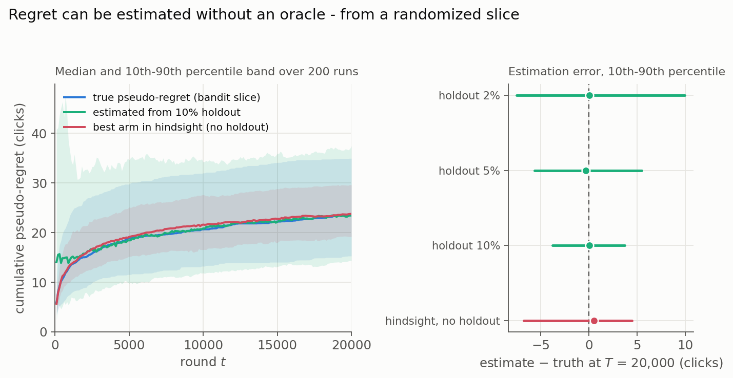
Holdout share	True regret of the bandit slice (median)	Estimate (median)	Estimation error, 10th to 90th percentile	Regret spent by the holdout itself (median)
2%	23.6	23.0	$-7.5$ to $+10.0$	53
5%	23.8	23.4	$-5.6$ to $+5.5$	133
10%	23.4	23.4	$-3.8$ to $+3.7$	268

Two things stand out. The estimate is unbiased at every holdout size (the median error is within a fraction of a click of zero), and its precision is set by the holdout, not by the bandit: with 10% of 20,000 rounds, each arm gets about 670 holdout impressions, each gap is known to about 0.02 (one standard error), and the error band is under four clicks either way. The last column is the price. The holdout is uniform allocation, so it pays a linear regret of $\tfrac{1}{3}(0.25 + 0.15) \approx 0.13$ expected clicks per holdout round: 268 clicks at 10%, more than ten times the 23 it is measuring. Measuring regret costs regret, and this bill is exactly fixed-$\epsilon$ greedy’s exploration bill from part 1 in another guise, because a uniform holdout is $\epsilon$-greedy’s exploration step, run beside a smarter exploiter.

That arithmetic explains why nobody runs a holdout in order to estimate regret. A holdout earns its keep by answering questions the bandit cannot answer about itself: whether its winner is still the winner under drift, what the losing arms are really worth, and whether the bandit beats plain randomization at all (compare reward per impression across the two slices, which is a two-sample test the earlier posts already covered). The regret estimate is a by-product, and a 2% to 5% slice buys most of it.

4.b) Best arm in hindsight, from the bandit’s own logs

The default on most dashboards skips the holdout: take the bandit’s own arm means, call the largest one $\hat{\mu}^\ast$, and plug into the same formula. The red curve and the bottom row of the figure show how that fares. In this example, surprisingly well: the median estimate lands within a click of the truth, with an error band ($-6.8$ to $+4.5$) about as wide as the 5% holdout’s, at zero cost. The reason is worth understanding, because it is also the reason not to trust it in general.

The error in arm $i$’s contribution is $N_i(T)$ times the error in $\hat{\mu}_i$, and the latter shrinks like $1/\sqrt{N_i(T)}$, so the contribution’s error grows only like $\sqrt{N_i(T)}$: the arms the bandit starved carry noisy means but small weights. Noise is self-limiting. Bias is not. The hindsight estimate measures regret against the bandit’s own belief about the best arm, so a bandit that has locked onto the wrong arm reports near-zero regret with complete confidence; a holdout would catch it. And the losing arms’ means carry the adaptive-sampling bias from section 3, which here shows up as an estimate about half a click too high (the red dot sitting right of zero). Well-separated arms hide that bias; nearly tied arms do not. When $\hat{\mu}^\ast$ is the maximum of two close, noisy estimates, it is biased upward by construction, and so is every gap built from it.

4.c) Proxies that do not pretend

When neither a holdout nor a propensity-logged exploration floor (section 3) is in place, an honest dashboard reports quantities that are actually observed and lets the reader infer, rather than an estimated regret with hidden assumptions:

• Share of traffic on the current leader, over time. The right panel of part 1’s shoot-out figure was exactly this, and it is computable in production.
• Exploration spend: traffic on non-leading arms times the leader’s lead in observed reward. This is the hindsight estimate presented as what it is, a bookkeeping figure.
• Realized reward per impression, bandit slice against holdout slice, when a holdout exists. This is the number that ends arguments.
• Time to concentration: rounds until the leader’s share crossed 90%, the operational version of “the regret curve bent”.

One habit ties these together, and it is the same one section 2 asked for: log the assignment probability, the chosen arm, the reward, and the resolution status per decision. With propensities logged and an exploration floor in place, the holdout’s unbiased means can be recovered from the bandit’s own traffic by inverse-propensity weighting, at the price of variance that grows as the floor shrinks. That is the bridge to the next post’s offline policy evaluation, where the same idea evaluates policies that were never run at all.

---

5. From One Global Winner to Personalization

Everything above shares one massive limitation: these algorithms find one global winner for everyone. Run Thompson Sampling on a streaming platform and it recommends the single most popular title to every user; run it on our campaign and it finds the best average CTR. But what if the short punchy ad wins on mobile during commutes, while the detailed one wins on desktop in the evening? Averaged over everyone, the two might look identical - and a vanilla bandit would see a tie where there is actually structure.

Learning which arm is best for this particular context is the contextual bandit problem, and it gets the next post to itself: the linear reward model, one fully hand-worked LinUCB decision, its Bayesian twin Linear Thompson Sampling, and the logging and fairness discipline personalization demands.

Onward to personalization.

---

Resources

• Joulani, P., György, A., and Szepesvári, C. (2013), “Online Learning under Delayed Feedback”, ICML - the stochastic-delay results behind section 2.
• Hadad, V., Hirshberg, D., Zhan, R., Wager, S., and Athey, S. (2021), “Confidence Intervals for Policy Evaluation in Adaptive Experiments”, PNAS, 118(15) - why adaptive data needs its own estimators (section 3).
• Lattimore, T. and Szepesvári, C. (2020), Bandit Algorithms, Cambridge University Press - the comprehensive, freely available reference behind both parts.