Contextual Bandits: Personalization with LinUCB and Linear Thompson Sampling

Part of the statistical-inference arc. It continues directly from multi-armed bandits, builds on causal inference, and closes into the GLM epilogue.

The previous post ended on a limitation: Thompson Sampling and UCB find one global winner for everyone. That is the right answer to the question they were asked - which arm is best on average? - but often the wrong question. This post asks the better one: which arm is best for this particular context?

That upgrade fuses supervised learning with exploration, and unlocks one of the workhorses of modern personalization (alongside supervised ranking and full sequential systems). We’ll build one running example, walk a complete decision through LinUCB with every matrix written out, replay the same decision through Linear Thompson Sampling, let both loose on a simulation, and close with the deployment discipline personalization demands: logging, offline evaluation, and fairness.

1. The Running Example: When the Global Winner Fails

A content site must choose, for each visitor, which of two article formats to show: a short-form summary, or the full technical deep-dive. These formats are our arms: serving one is a pull, as showing an ad was before.

Before deciding, we see one clue about the visitor: their context. Here it is a single number, a session-intent score $z \in [-1, 1]$, computed from signals available when the page is requested (referrer, time of day, device): low $z$ suggests a hit-and-run visit, high $z$ a settled one. In our toy environment visitors arrive with $z \sim \text{Uniform}(-1, 1)$ - a choice made for clean arithmetic, not a fact about real intent scores, and every “average over visitors” below leans on it.

The reward is a standardized engagement score (a blend of scroll depth and dwell time): a real-valued index typically between 0 and 1, not a clamped fraction, observed only for the format actually served. Unknown to the learner, the true expected rewards are straight lines in $z$:

\[\mu_{\text{short}}(z) = 0.55 - 0.20\,z, \qquad \mu_{\text{deep}}(z) = 0.55 + 0.20\,z\]

Observed rewards scatter around those lines: serving format $a$ at intent $z$ returns $\mu_a(z)$ plus $\mathcal{N}(0, 0.1^2)$ noise. (Gaussian tails are why the score must stay unbounded - and keeping the noise honestly Gaussian keeps every later formula exact.)

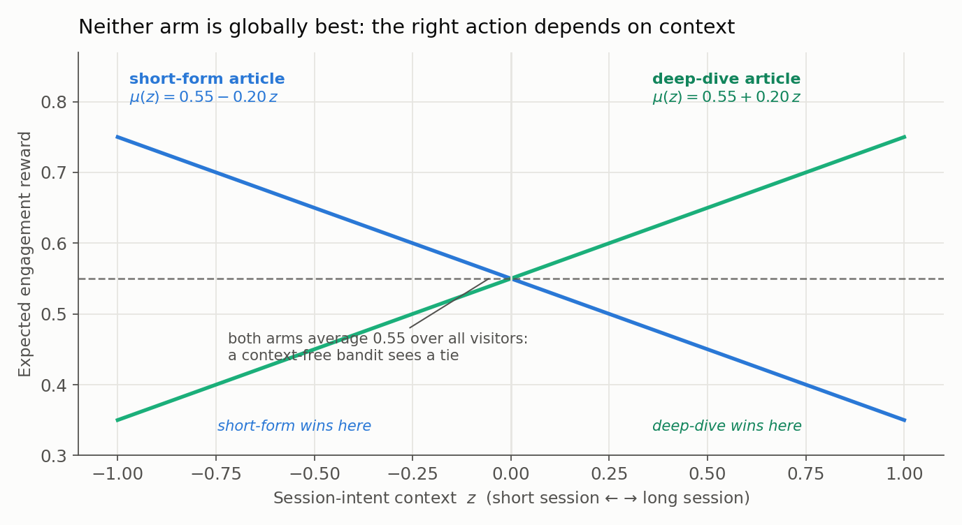
The dashed line is the punchline. Averaged over the uniform visitor population, both arms earn exactly 0.55: a vanilla bandit, which only tracks per-arm averages, would grind toward a coin-flip and see nothing left to learn. Yet at $z = -0.8$ the short-form is better by 0.32, at $z = +0.8$ the deep-dive is: all the structure lives in the context, and a context-free learner is blind to it. (The engineered tie needs both the symmetric lines and the symmetric context distribution - skew the visitor mix and the averages separate - but a milder version plays out whenever the lines cross where visitors occur.)

The size of the prize. Any fixed-arm policy earns 0.55 per visitor: the ceiling for every context-blind strategy. The rule the figure suggests - deep-dive when $z > 0$, short-form when $z < 0$ - earns the winning line, $0.55 + 0.20 \lvert z \rvert$, and averaging it needs $\mathbb{E}\lvert z \rvert$: the uniform density on an interval of length 2 is $\tfrac{1}{2}$ everywhere, and taking absolute values folds the left half onto the right, leaving $\lvert z \rvert$ uniform on $[0,1]$ with mean one half:

\[\mathbb{E}\lvert z \rvert = \int_{-1}^{1} \lvert z \rvert \cdot \tfrac{1}{2}\, dz = 2 \int_{0}^{1} z \cdot \tfrac{1}{2}\, dz = \frac{1}{2}\] \[\Rightarrow \quad \mathbb{E}\big[\,0.55 + 0.20\,\lvert z \rvert\,\big] = 0.55 + 0.20 \cdot 0.5 = 0.65\]

The ideal split earns 0.65 per visitor against 0.55 for the best fixed arm: a lift of roughly 18% that no vanilla bandit can capture. The lift comes from cutting exactly at the crossover - cut at $z = 0.3$ instead and the band between 0 and 0.3 leaks reward; learning where to cut is precisely the contextual bandit’s job.

What is actually being learned. It is tempting to picture the algorithm learning that routing rule directly (“send $z > 0$ to the deep-dive”). The algorithms in this post never do: they learn only the arms’ reward equations - their working estimates of the two lines - and re-derive each choice by evaluating both lines at the visitor’s $z$ (the model-based family; other methods do learn a policy or value function directly). The boundary is emergent - simply where the estimates cross, shifting whenever new data bends a line - and one nuance carries through the post: each equation is learned accurately only where its arm gets played, a regression in service of a ranking.

Why not segment-and-run-two-bandits? Splitting at $z = 0$ presumes we already know the threshold - exactly what we do not know. And real context is continuous and multi-dimensional: slicing it into cells fragments the data and hard-codes boundaries we should be learning. The contextual bandit instead shares information across the context space through a model.

A design note. We deliberately use a behavioral, session-level feature rather than a demographic one: demographic features can encode or proxy protected attributes, and a reward-optimizing policy will happily exploit them - feature choice is a fairness and privacy decision, not only a modeling one, and even session signals can act as proxies (section 7 returns to this). The continuous reward is deliberate too: it keeps the linear-Gaussian machinery honest, while binary rewards call for a logistic bandit - the bridge to the GLM epilogue.

How One Round Plays Out, in Plain Words

This post is denser than the last (matrices ahead), so here is the entire mechanism narrated once:

1. A visitor arrives; we look at the context first. Their session signals score $z = 0.5$: probably a settled visit.
2. Each arm predicts its reward for this visitor. The policy keeps a working guess of each arm’s reward line; read at $z = 0.5$: short-form about 0.45, deep-dive about 0.65.
3. Each prediction carries a confidence tag. Plenty of deep-dives have gone to low-intent visitors but few to high-intent ones, so the deep-dive guess out here is shaky: uncertainty depends on where the visitor sits, not just how often an arm was played.
4. Prediction and uncertainty combine into a choice. LinUCB adds an optimism bonus sized by the uncertainty; Linear Thompson Sampling wobbles each line within its uncertainty and trusts the wobble. Either way, an arm that might be great here gets a real chance to prove it.
5. We serve the winner and watch. The deep-dive is chosen; the visitor engages at 0.71.
6. Only the served arm learns. Its line is tugged toward the observation and its uncertainty there shrinks; the short-form learned nothing. That missing “what if” is the defining constraint of the whole problem.

Repeat thousands of times and the guessed lines bend toward the true ones; the choices sharpen into a rule: short-form below the crossover, deep-dive above. The sections that follow make each step precise.

Relative to the previous post: partial feedback, the explore-exploit dilemma, and update-only-the-played-arm are untouched. What changed is the object being learned - a context observed before choosing, a function $\mu(x, a) = x^\top \theta_a$ per arm instead of one number, a context-dependent “best arm” and regret benchmark, uncertainty as a curve over the context space - and that is why this post needs its own machinery.

---

2. Formalizing the Contextual Bandit

At each round $t$:

1. Observe the context $x_t$ (features available before acting).
2. Choose an arm $a_t$.
3. Observe the reward $r_t$ only for the chosen arm.
4. Update the policy and wait for the next round.

Step 3 separates this from supervised learning and deserves a name: partial feedback. A supervised dataset would reveal how both formats performed for every visitor; our log contains only the road taken, and the counterfactual reward is permanently missing. Two consequences shape everything below:

• We must still explore. Stop serving the deep-dive to low-intent visitors and we stop learning about it there; a wrong early impression can never be corrected.
• Our own past choices shape our own data. The training data is whatever our earlier decisions collected - the last post’s adaptive-collection problem with context attached, and the reason for section 7’s logging discipline.

Instead of one number $\mu_a$ per arm, we estimate a function $\mu(x, a)$: the expected reward of arm $a$ given context $x$.

---

3. The Shared Linear Reward Model

Both algorithms assume the same reward model. For our one-feature example, the context vector for visitor $t$ is

\[x_t = \begin{bmatrix} 1\\ z_t \end{bmatrix}, \qquad \mathbb{E}[r_t \mid x_t, a] = x_t^\top \theta_a\]

In words: each arm’s expected reward is a straight line in the context, and $x_t^\top \theta_a$ simply evaluates that line - intercept plus slope times $z_t$. Each arm owns its own pair $\theta_a = (\theta_{a,0}, \theta_{a,1})^\top$:

• $\theta_{a,0}$, the intercept: the arm’s expected reward for an average-intent ($z = 0$) visitor; the constant 1 in $x_t$ buys this degree of freedom.
• $\theta_{a,1}$, the slope: how strongly reward responds to intent. In truth $\theta_{\text{short}} = (0.55, -0.20)$ and $\theta_{\text{deep}} = (0.55, +0.20)$; the learner must estimate both from partial feedback.
• The arms get separate parameters (the disjoint model) because nothing says the two formats respond to intent the same way; the separation is what lets fitted lines cross.

One idea changes shape. In the previous post an arm’s uncertainty was a single number that shrank with pulls; here uncertainty lives in the context space: the same arm can be precisely understood at low $z$ (where it has data) and nearly unknown at high $z$ (where it has none), an exploit choice for one visitor and an explore choice for the next. That is the geometric heart of everything below.

---

4. Worked Example: LinUCB

LinUCB transplants “optimism under uncertainty” into the linear model, fitting each arm’s line by ridge regression: least squares plus a mild stabilizer $\lambda$ that keeps the fit sensible before much data exists (we use $\lambda = 1$). The whole algorithm rests on two objects per arm:

\[A_a = \lambda I + \sum_{s:\, a_s = a} x_s x_s^\top, \qquad b_a = \sum_{s:\, a_s = a} r_s x_s\]

The notation first: $s$ counts rounds, and $s : a_s = a$ under each sum reads “keep only the rounds where this arm was played” - each arm’s sums come purely from its own serving history. And the formulas are not new machinery: stack arm $a$’s served contexts as rows of $X$ and its rewards in $r$, and the textbook ridge closed form $\hat{\theta} = (X^\top X + \lambda I)^{-1} X^\top r$ expands row by row into exactly $A_a$ and $b_a$: the outer product $x_s x_s^\top$ is simply $X^\top X$ accumulated one observation at a time, which lets the bandit fold each visitor in without refitting. For $x_s = (1, z_s)^\top$ it collapses into plain bookkeeping:

\[x_s x_s^\top = \begin{bmatrix} 1 & z_s\\ z_s & z_s^2 \end{bmatrix} \;\Rightarrow\; A_a = \lambda I + \begin{bmatrix} n_a & \sum z_s\\ \sum z_s & \sum z_s^2 \end{bmatrix}, \qquad b_a = \begin{bmatrix} \sum r_s\\ \sum r_s z_s \end{bmatrix}\]

So $A_a$ stores how often the arm was played ($n_a$), where its contexts sat ($\sum z_s$), and how spread they were ($\sum z_s^2$); $b_a$ stores the total reward and where it was earned: $A_a$ remembers where the arm has been tried, $b_a$ what happened there. Together they are everything the model needs (its sufficient statistics), though raw logs stay necessary for drift diagnostics, delayed rewards, and section 7’s offline evaluation. Fitting and scoring take one step each:

\[\hat{\theta}_a = A_a^{-1} b_a, \qquad p_a(x) = \underbrace{x^\top \hat{\theta}_a}_{\text{predicted reward}} \;+\; \alpha \, \underbrace{\sqrt{x^\top A_a^{-1} x}}_{\text{uncertainty at } x}\]

The bonus term $\sqrt{x^\top A_a^{-1} x}$ is a geometric uncertainty width: how far this visitor’s $x$ sticks out into directions where the arm has little data. LinUCB multiplies it by a confidence radius $\alpha$ to form a high-probability upper bound on the arm’s expected reward at $x$: “prediction plus $\alpha$ uncertainty widths”, the same recipe as the previous post’s UCB. The width behaves like a standard error, with one honesty note: under ridge regularization and adaptively collected data it is not literally the conventional fixed-design standard error - the rigorous justification is the self-normalized concentration analysis of Abbasi-Yadkori, Pál, and Szepesvári (2011), whose radius folds the noise scale, parameter norm, dimension, and failure probability into what practitioners tune as $\alpha$. The appendix untangles which covariance is which.

One consequence makes the formula feel inevitable: strip the context away and the inverse-count geometry reappears. With no features, $A_a$ collapses to $n_a + \lambda$ and the width to $1/\sqrt{n_a + \lambda}$ - the $1/\sqrt{n}$ shape of the previous post’s bonus (not the full UCB1 rule; its $\sqrt{\ln t}$ schedule played the role $\alpha$ plays here). The matrix generalizes “number of pulls” to “amount of data in this visitor’s direction”; the appendix’s eigen-view makes the pricing exact.

(Two conventions. We display $A_a^{-1}$ because the $2 \times 2$ arithmetic is instructive; production code solves linear systems instead. And $A_a = \lambda I$ shrinks the intercept along with the slope - standard practice, but as a prior belief (“baseline reward 0”) knowingly wrong here; centering rewards, or a nonzero prior mean, is the remedy when it matters.)

4.a) The State After 12 Rounds

Twelve visitors have been served, six per arm. The full history (context $z$, observed reward $r$):

Rounds where the short-form was shown:

Context $z$	$-0.9$	$-0.6$	$-0.3$	$0.0$	$0.3$	$0.8$
Reward $r$	$0.78$	$0.61$	$0.65$	$0.50$	$0.45$	$0.42$

Rounds where the deep-dive was shown:

Context $z$	$-0.8$	$-0.7$	$-0.5$	$-0.2$	$0.0$	$0.3$
Reward $r$	$0.35$	$0.46$	$0.42$	$0.55$	$0.59$	$0.66$

Notice the deep-dive arm’s data problem before any algebra: all six observations sit at $z \le 0.3$ - early traffic skewed low-intent, so the model knows the deep-dive well on the left and hardly at all on the right.

Accumulating the sums (with $\lambda = 1$) - every entry checkable from the tables: six pulls plus $\lambda$ makes the 7, contexts sum to $-0.70$, squares to $1.99$ plus $\lambda$ giving $2.99$:

\[A_{\text{s}} = \begin{bmatrix} 7 & -0.70\\ -0.70 & 2.99 \end{bmatrix}, \quad b_{\text{s}} = \begin{bmatrix} 3.41\\ -0.792 \end{bmatrix} \;\Rightarrow\; \hat{\theta}_{\text{s}} = A_{\text{s}}^{-1} b_{\text{s}} = \begin{bmatrix} 0.472\\ -0.155 \end{bmatrix}\]

and for the deep-dive arm:

\[A_{\text{d}} = \begin{bmatrix} 7 & -1.90\\ -1.90 & 2.51 \end{bmatrix}, \quad b_{\text{d}} = \begin{bmatrix} 3.03\\ -0.724 \end{bmatrix} \;\Rightarrow\; \hat{\theta}_{\text{d}} = A_{\text{d}}^{-1} b_{\text{d}} = \begin{bmatrix} 0.446\\ 0.049 \end{bmatrix}\]

Both estimates sit closer to zero than the truths $(0.55, -0.20)$ and $(0.55, +0.20)$: partly the stabilizer, partly just six noisy points each. The deep-dive slope (0.049 vs. a true 0.20) is the interesting one: bunched on the left, it is only weakly identified - a narrow context range does not force underestimation, but it leaves the fit at the mercy of ridge shrinkage and noise, which in this sample land it well below the truth. The right half of the line is guesswork stretched out from the left.

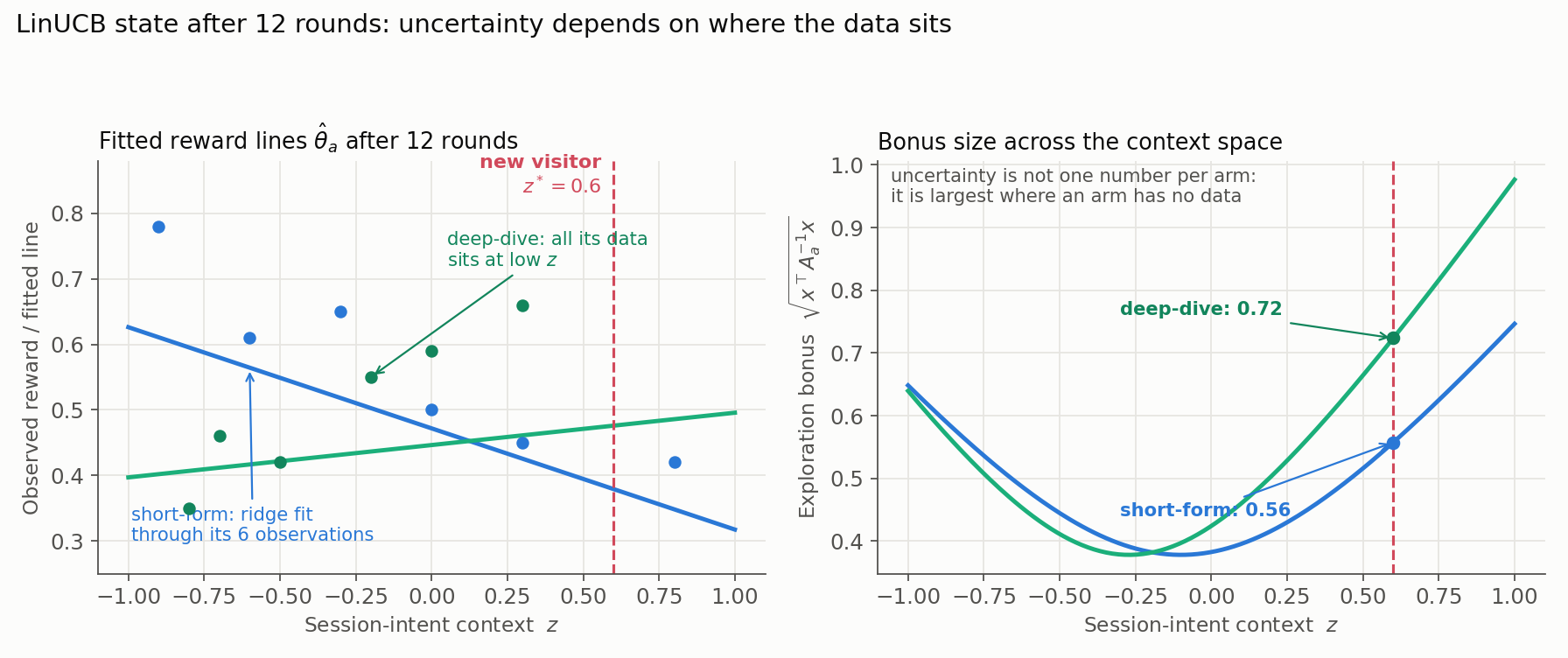
The right panel is the new idea made visible: the exploration bonus is a curve over the context space, not a number. Both arms are confident near $z \approx -0.3$ where their data clusters, and the deep-dive arm, whose data sits further left, is markedly more uncertain on the right half.

4.b) One Decision, Every Number Shown

A new visitor arrives with $z^\ast = 0.6$, so $x^\ast = (1, 0.6)^\top$. We use $\alpha = 1$.

Quantity	Short-form	Deep-dive
Predicted reward $x^{\ast \top} \hat{\theta}_a$	$0.472 - 0.155 \cdot 0.6 = 0.379$	$0.446 + 0.049 \cdot 0.6 = 0.476$
Uncertainty $\sqrt{x^{\ast \top} A_a^{-1} x^\ast}$	$0.557$	$0.724$
LinUCB score $p_a(x^\ast)$	$0.936$	$\mathbf{1.200}$ ✓
(True expected reward, hidden)	$0.430$	$0.670$

The deep-dive wins on both components: a slightly higher prediction and a much larger bonus, precisely because it has never been tried out here. This is optimism acting per-visitor: for this visitor the deep-dive is an exploration play; at $z = -0.5$, where its data lives, it would score almost purely on prediction.

The observation and update. We serve the deep-dive; the visitor returns $r = 0.72$. Only the played arm’s state changes:

\[A_{\text{d}} \leftarrow A_{\text{d}} + x^* x^{*\top} = \begin{bmatrix} 8 & -1.30\\ -1.30 & 2.87 \end{bmatrix}, \qquad b_{\text{d}} \leftarrow b_{\text{d}} + 0.72\, x^* = \begin{bmatrix} 3.75\\ -0.292 \end{bmatrix}\] \[\hat{\theta}_{\text{d}} = A_{\text{d}}^{-1} b_{\text{d}} = \begin{bmatrix} 0.488\\ 0.119 \end{bmatrix}\]

One well-placed observation moved the slope estimate from 0.049 to 0.119, halfway to the truth: a point at $z = 0.6$ is highly informative about a line anchored only on the left. The uncertainty at $z^\ast$ drops from 0.724 to 0.586, and the shrinkage is directional: adding $x^\ast x^{\ast\top}$ is a rank-one update, so uncertainty falls most for contexts pointing the same way as $x^\ast$ (the whole high-intent half benefits) and least elsewhere. The next high-intent visitor will find the deep-dive scored more on evidence, less on optimism.

---

5. Worked Example: Linear Thompson Sampling

Now the Bayesian twin: the same historical state ($A_a$, $b_a$ after 12 rounds), the same visitor $z^\ast = 0.6$, only the decision rule changed.

Before, Thompson Sampling played the arm with the largest value sampled from its Beta posterior. Linear Thompson Sampling lifts the idea one level: each arm’s belief is now about its whole line, a cloud of plausible intercept-slope pairs dense near the best fit and thinning outward:

\[\theta_a \mid \mathcal{D} \;\sim\; \mathcal{N}\!\left(\hat{\theta}_a,\; \sigma^2 A_a^{-1}\right)\]

This is not an invented analogue of LinUCB; it is a theorem. Give $\theta_a$ a Gaussian prior centered at zero - exactly the Bayesian reading of the ridge stabilizer, $\lambda = \sigma^2/\tau^2$ for a prior of width $\tau$ - and assume Gaussian reward noise. Then conjugacy (Beta-Bernoulli’s Gaussian sibling) gives an exactly Gaussian posterior whose mean is the ridge estimate $\hat{\theta}_a$ and whose covariance is $\sigma^2 A_a^{-1}$: this is Bayesian linear regression, derived in the appendix, and it is what makes the post cohere - section 4’s bonus matrix is this posterior covariance, up to the noise scale. LinUCB adds a multiple of the width deterministically; Linear TS samples from the belief it encodes.

In practice, implementations sample from $\mathcal{N}(\hat{\theta}_a, v^2 A_a^{-1})$ with a tunable $v$ in the slot the theorem assigns to $\sigma$. We use $v = 0.15$ against true noise $\sigma = 0.10$, so what we sample is - by its right name - not the exact posterior but a deliberately inflated, posterior-shaped exploration distribution. The inflation is standard: $\sigma$ is unknown in practice, under-estimating it is the dangerous direction (too-tight clouds stop exploring too early), and formal analyses (Agrawal and Goyal, 2013) inflate further still for their guarantees. A draw $\tilde{\theta}_a$ is one plausible reward line: where the arm has data all draws nearly agree; where it has none, they fan out:

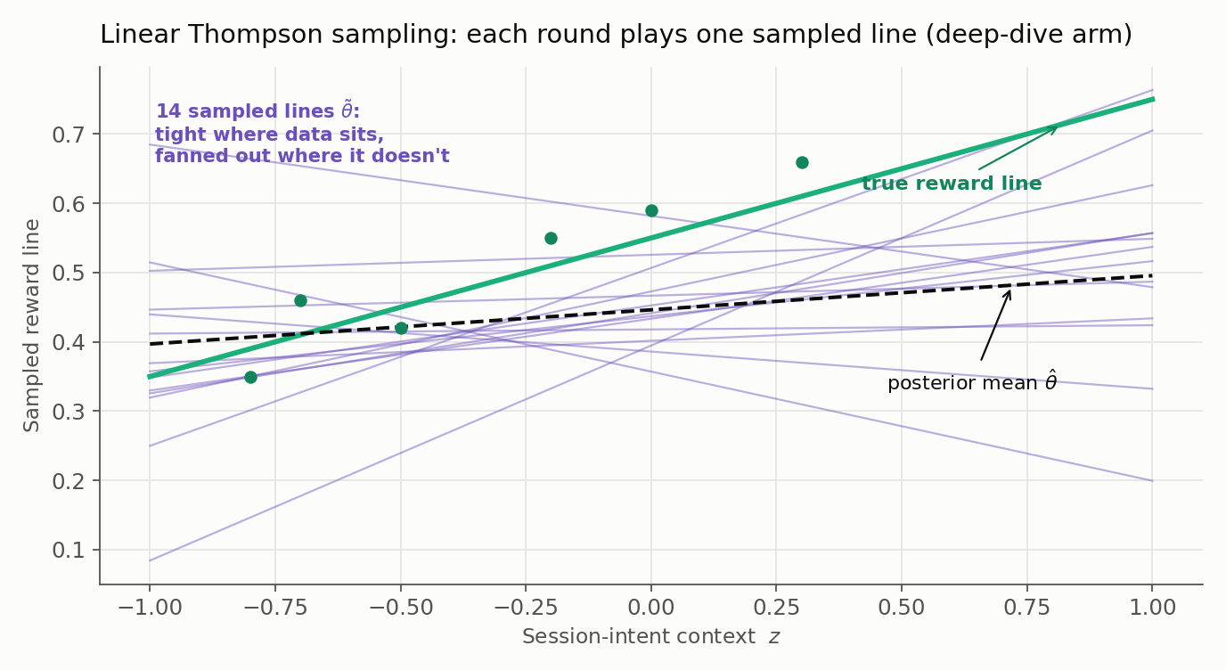
The fan-out on the right is the exploration mechanism, as the wide Beta posterior was before: no bonus is computed; uncertainty becomes exploration through randomness.

The same decision, replayed. For each arm:

1. Draw from each cloud: $\tilde{\theta}_{\text{s}} = (0.466, -0.142)$, $\tilde{\theta}_{\text{d}} = (0.476, 0.114)$.
2. Score the visitor on the sampled line: $x^{\ast \top} \tilde{\theta}_{\text{s}} = 0.466 - 0.142 \cdot 0.6 = 0.381$, and $x^{\ast \top} \tilde{\theta}_{\text{d}} = 0.476 + 0.114 \cdot 0.6 = \mathbf{0.545}$ ✓.
3. Play the largest: the deep-dive again, then update $A_{\text{d}}, b_{\text{d}}$ exactly as in LinUCB (posterior and ridge updates are the same bookkeeping).

Note what randomness bought and cost. The deep-dive’s sampled slope (0.114) landed above its posterior mean (0.049), so this draw leaned optimistic much like LinUCB’s bonus - but a rerun could sample a pessimistic line and serve the short-form instead. Given identical histories, LinUCB’s next action is fixed; Linear Thompson’s is a random variable reflecting its (deliberately inflated) posterior-shaped beliefs. (Naming: this Gaussian recipe is one common implementation, hence Linear Thompson Sampling; the general contextual version samples from whatever posterior the reward model maintains.)

LinUCB vs. Linear Thompson Sampling

Question	LinUCB	Linear Thompson Sampling
Uncertainty	Confidence ellipsoid around $\hat{\theta}_a$	Posterior distribution over $\theta_a$
Exploration	Deterministic bonus $\alpha \sqrt{x^\top A_a^{-1} x}$	Random parameter sample $\tilde{\theta}_a$
Same history, same next action?	Always	Not necessarily
Prior knowledge	Less direct (initialize $A_a, b_a$)	Natural (it is a prior)
Main tuning	Exploration coefficient $\alpha$	Prior/noise scale $v$

---

6. Simulation: Watching the Policy Materialize

We now run both algorithms from scratch: $z \sim \text{Uniform}(-1,1)$, rewards off the true lines plus unclipped Gaussian noise, 2,500 rounds per run, 200 seeded simulations, pointwise medians with 10th-90th percentile bands. Within each seed all policies replay the same visitor stream, with the algorithms exactly as specified above (disjoint models, $\lambda = 1$, $\alpha = 1$, $v = 0.15$, intercept included and regularized).

One definition needs upgrading. We plot contextual pseudo-regret: each round charges the gap between the best arm’s expected reward at that context and the chosen arm’s,

\[\bar{R}_T = \sum_{t=1}^{T} \Big[ \max_a \mu(x_t, a) - \mu(x_t, a_t) \Big]\]

Serving the short-form at $z = 0.7$ costs $0.28$ even though the short-form is great elsewhere; the benchmark is section 1’s 0.65 oracle, not its 0.55 fixed-arm ceiling, so a policy can match the best fixed arm and still bleed regret on every wrongly-served visitor. And only the simulator, which knows both true lines, can compute it; a production log sees one noisy reward for the action taken - the bracketed counterfactual is what partial feedback withholds.

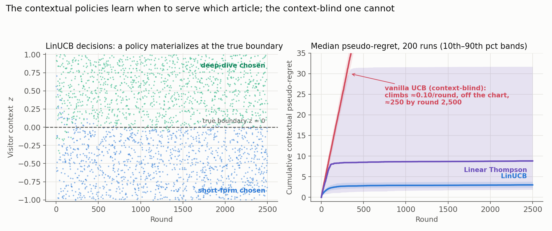
The left panel is the post’s central visual. A decision boundary materializes along the true crossover $z = 0$: the policy has learned a rule, “deep-dive above, short-form below”, from partial feedback alone. Over its final 500 rounds LinUCB serves the context-optimal arm 99.8% of the time (one seed’s showing, not a guarantee). The pseudo-regret curves grow increasingly slowly, and the simulation demonstrates something stronger than before: the policy is right conditionally on context, not just on average.

The third curve, the previous post’s vanilla UCB dropped into this environment, is the cautionary tale of the series. Ignoring $z$, it experiences the two arms as a true tie and splits traffic 50/50 forever - and by its own scorecard it is doing perfectly: about 0.55 per visitor, matching the best fixed arm, vanilla regret essentially zero. Re-scored against the contextual benchmark, the same decisions leak $\mathbb{E}[0.20 \lvert z \rvert] = 0.10$ per round: a straight line to roughly 250 while the contextual policies sit below ten. No metric vanilla UCB tracks would reveal the problem - the failure is visible only under the right regret definition - and section 1’s dashed-line tie becomes a trajectory: “no significant difference” in an aggregate test can coexist with strong, opposite preferences across segments.

Two honest footnotes. First, the tunings matter: with $\alpha = 1$ and $v = 0.15$, LinUCB’s median pseudo-regret ($\approx 3.0$) beats Linear Thompson’s ($\approx 8.8$) with a far tighter band, but cranking $v$ down or $\alpha$ up can flip the picture - a property of the tuning pair, not a theorem. And Linear Thompson’s 90th-percentile edge ($\approx 32$) sits several times above its median: a downside tail the median hides, which an operational choice might weigh heavily. Second, this environment is easy - exactly linear, one feature, stationary, instant feedback - and real deployments are messier along every axis: the next section’s subject.

---

7. Deployment and Evaluation: The Discipline Personalization Demands

The previous post established why adaptive collection corrupts naive inference and listed operational guardrails (traffic floors, kill switches, ramp-ups). Context raises the stakes: assignment probabilities now depend on who the visitor is, and the after-the-fact questions are about policies, not arms.

Log enough to reconstruct every decision. For each round, record:

• the context $x_t$ as seen at decision time, plus model version and hyperparameters;
• the eligible action set and the chosen action;
• the propensity: the probability the policy assigned to each eligible action. Linear TS’s probability is well-defined but a realized draw does not reveal it - it must be computed (a closed form on the difference of sampled scores here: 0.76 for the worked visitor; Monte Carlo for richer policies); deterministic LinUCB needs one created by an exploration floor (a random eligible arm with probability $\varepsilon_{\min}$). Logging the seed is no substitute for the probability;
• the observed reward, its delay, and any guardrail outcomes.

Offline policy evaluation (OPE). The log lets us estimate how a new policy would have performed without deploying it. The core trick is inverse propensity scoring (IPS): reweight each logged round by how much more often the new policy would have taken the logged action than the old one did,

\[\hat{V}_{\text{IPS}}(\pi_{\text{new}}) = \frac{1}{T} \sum_{t=1}^{T} \frac{\pi_{\text{new}}(a_t \mid x_t)}{\pi_{\text{old}}(a_t \mid x_t)} \, r_t\]

The catch: IPS is honest only if every action the new policy might take had some chance of being logged; an exploration floor is one way to guarantee that coverage. Overlap is necessary, not sufficient: honest OPE also needs correctly logged propensities and eligible sets, decision-time contexts, resolved delayed rewards, and held-out data or cross-fitting when the candidate policy was trained on the log now scoring it. IPS’s other cost is noise: rarely-logged actions get enormous weights. The remedy is the doubly robust estimator of Dudík, Langford, and Li (2011), pairing IPS with a fitted reward model: consistent if either ingredient is correct, and since a logged bandit normally knows its own propensities, the reward model’s main gift is variance reduction. It is a close relative of the propensity-score machinery in the causal-inference post, aimed at whole policies rather than one treatment effect.

The moving parts to monitor. Context drift, reward drift, and delayed or censored rewards all quietly violate the stationary, instant-feedback assumptions; production systems answer with sliding windows or discounting, pending-outcome accounting, and explicit missingness handling.

Feature governance. Two rules apply with extra force:

• No post-treatment features. Context must predate the action (time-on-page so far qualifies; time-on-page after serving is leakage that destroys the reward model’s meaning) - and if earlier recommendations shaped that pre-action state, today’s action influences tomorrow’s context, drifting toward section 8’s sequential setting.
• Feature selection is a fairness and privacy decision. A contextual policy is a machine for treating people differently based on their features; features that encode or proxy protected attributes can produce unfair treatment while optimizing reward perfectly. Hence session intent in our example (with section 1’s proxy caveat), and audits beyond realized treatment rates: conditional treatment probabilities, reward and error disparities across groups, and proxy-feature analysis.

---

8. Where the Linear Assumption Breaks

Everything above leaned on $\mathbb{E}[r \mid x, a] = x^\top \theta_a$. Four ways reality outgrows it, in increasing order of machinery:

• Binary rewards → logistic bandits. A linear model of a click probability can predict values outside $[0, 1]$. (Not automatically invalid - it works when the true mean is genuinely linear and stays in range over the contexts that occur - but fragile outside that domain.) The fix passes the score through a link function, a GLM bandit with the logistic link guaranteeing the range: the exact bridge to the epilogue, where the same GLMs that unify t-tests and proportion tests generalize these bandits.
• Nonlinear structure. Interactions (deep-dives win for high-intent visitors only on desktop) need engineered features or a richer function class: tree ensembles, or neural bandits - which do not carry usable uncertainty for free the way the linear-Gaussian model did; exploration then needs an explicit mechanism grafted on (bootstrapped ensembles, Bayesian last layers, or similar).
• Combinatorial actions. A slate of five articles is not five independent choices (they cannibalize each other’s clicks); combinatorial bandits handle structured action spaces.
• Actions that change the future → full RL. When today’s action alters tomorrow’s context (ad fatigue, content burnout, habit formation), we have left bandits for Markov Decision Processes and reinforcement learning. Contextual bandits are often called “one-step RL” - the defining assumption being that actions do not change future decision states in a way the policy must plan around - and knowing which side of the line a problem sits on is itself a design decision.

---

Where This Leaves Us (and the Epilogue Ahead)

From p-value to personalized decision boundary, the series has traced the full arc of experimentation: estimating an effect under clean randomization, recovering effects without it (causal inference), optimizing reward while learning (multi-armed bandits), and now personalizing the decision itself - with stopping rules and power (sample-size planning) recurring throughout.

One question ties it together: a t-test assumes roughly normal outcomes, a proportion test binary ones, and this post modeled a continuous score with a linear function while flagging binary rewards as favoring a link function. Is there one modeling language for continuous, binary, and count outcomes alike? There is: the short epilogue on generalized linear models that closes the series.

Happy experimenting - onward to the epilogue.

---

Resources

• Li, Chu, Langford, and Schapire (2010), A Contextual-Bandit Approach to Personalized News Article Recommendation - introduced LinUCB.
• Abbasi-Yadkori, Pál, and Szepesvári (2011), Improved Algorithms for Linear Stochastic Bandits - the confidence-ellipsoid analysis behind the bonus.
• Agrawal and Goyal (2013), Thompson Sampling for Contextual Bandits with Linear Payoffs - Linear TS guarantees, with the inflated sampling scale.
• Dudík, Langford, and Li (2011), Doubly Robust Policy Evaluation and Learning - doubly robust offline policy evaluation.

---

Appendix: Why the Bonus Measures an Uncertain Direction

Section 4 called $\sqrt{x^\top A_a^{-1} x}$ an uncertainty width rather than a conventional standard error. Three related but distinct facts share the matrix $A^{-1}$; keeping them separate is the point (one fixed arm; subscripts dropped).

Fact 1: the frequentist sampling covariance of the ridge estimate is not $\sigma^2 A^{-1}$. With the arm’s contexts stacked as rows of $X$, rewards in $r$, model $r = X\theta + \varepsilon$, $\text{Cov}(\varepsilon) = \sigma^2 I$, and $A = X^\top X + \lambda I$:

\[\hat{\theta} = A^{-1} X^\top r = A^{-1} X^\top X \theta + A^{-1} X^\top \varepsilon\]

The first term is deterministic ($\theta$ itself only at $\lambda = 0$; the small ridge bias is the price of stability); all randomness sits in the second, so $\text{Cov}(M\varepsilon) = M \, \text{Cov}(\varepsilon) \, M^\top$ gives:

\[\text{Cov}(\hat{\theta}) = \sigma^2 A^{-1} (X^\top X) A^{-1} = \sigma^2 \left( A^{-1} - \lambda A^{-2} \right)\]

Only at $\lambda = 0$ does $X^\top X = A$ collapse this to $\sigma^2 A^{-1}$. With ridge the two matrices differ, most (relatively) along data-starved directions - exactly the ones that drive exploration. Through the prediction, $\text{Var}(x^\top \hat{\theta}) = x^\top \text{Cov}(\hat{\theta})\, x$: for the worked visitor with $\sigma = 0.10$, frequentist standard errors of $\approx 0.047$ (short-form) and $0.051$ (deep-dive) versus $\sigma \sqrt{x^\top A^{-1} x}$ of $0.056$ and $0.072$. The bonus is the larger, more cautious width, most so for the data-poor arm - the safe direction to err in, but not the same number.

Fact 2: what actually justifies LinUCB. Fact 1 still conditions on $X$ as a fixed design, but a bandit’s design depends on its own earlier rewards. The rigorous theory (Abbasi-Yadkori, Pál, and Szepesvári, 2011) instead bounds the estimation error in the $A$-norm using self-normalized martingale concentration, valid under adaptive collection; that bound licenses “prediction plus radius times $\sqrt{x^\top A^{-1} x}$” as a high-probability statement. The geometry survives; the constant comes from this theory.

Fact 3: the Bayesian posterior covariance is exactly $\sigma^2 A^{-1}$. Treat the same model as Bayesian linear regression: prior $\theta \sim \mathcal{N}(0, \tau^2 I)$, likelihood $r \mid \theta \sim \mathcal{N}(X\theta, \sigma^2 I)$. Gaussian precisions (inverse covariances) add, the data contributing $X^\top X / \sigma^2$:

\[\Sigma_{\text{post}}^{-1} = \frac{X^\top X}{\sigma^2} + \frac{I}{\tau^2} = \frac{1}{\sigma^2} \left( X^\top X + \frac{\sigma^2}{\tau^2} I \right) = \frac{A}{\sigma^2} \quad \text{with } \lambda = \frac{\sigma^2}{\tau^2}\] \[\Rightarrow \quad \Sigma_{\text{post}} = \sigma^2 A^{-1}, \qquad \mu_{\text{post}} = \Sigma_{\text{post}} \frac{X^\top r}{\sigma^2} = A^{-1} X^\top r = \hat{\theta}\]

So the ridge estimate is the posterior mean, the ridge penalty is the prior (wide prior, small $\lambda$) - and it is this covariance, not Fact 1’s, that equals $\sigma^2 A^{-1}$ exactly. One matrix, two philosophies: LinUCB adds a multiple of the width, leaning on Fact 2 for rigor; Linear TS samples from Fact 3’s posterior (inflated, per section 5); Fact 1 agrees only at $\lambda = 0$. For the full Bayesian machinery, including the predictive distribution and lasso via the Laplace prior, see Bayesian linear regression.

The eigen-view. Diagonalizing the scatter matrix $A = V \Lambda V^\top$ (eigenvectors $v_i$, eigenvalues $\lambda_i$) turns the quadratic form into a priced sum over directions:

\[x^\top A^{-1} x = \sum_i \frac{(v_i^\top x)^2}{\lambda_i}\]

Each direction charges the squared overlap of $x$ with it, priced inversely to the data along it - large-eigenvalue directions cheap, small ones expensive. In section 4.a’s deep-dive state, $A_{\text{d}}$ has eigenvalues $\approx 7.7$ and $\approx 1.8$, the starved direction pointing toward high $z$ - exactly why the $z^\ast = 0.6$ visitor drew the large 0.72 bonus.