Bayesian Linear Regression: Where Ridge and Lasso Come From

A Bayesian coda to the linear-regression series (Part 1, Part 2, Part 3). It builds on the Normal and Laplace distribution posts and the conjugacy ideas from the Beta post.

Our linear-regression series introduced Ridge and Lasso as stabilizers: penalties bolted onto the loss to tame multicollinearity and shrink overfit coefficients, with a passing mention that both have Bayesian readings. This post makes good on that mention, because the Bayesian reading answers a question most practitioners have wondered about at some point: why those penalties? Ridge adds a sum of squares to the loss, lasso adds a sum of absolute values, and both look like tricks someone invented to stop overfitting.

They are not tricks. Both penalties are priors wearing a disguise: ridge is what a Gaussian prior on the coefficients looks like from the outside, and lasso is what a Laplace prior looks like. This post makes that identity precise, works one posterior end to end by hand, and shows what the Bayesian view buys beyond a justification: a fit that carries its posterior and predictive uncertainty with it.

1. What a Point Estimate Leaves Out

Ordinary least squares picks the coefficients that minimize the residual sum of squares. Our linear-regression series covers the mechanics and the frequentist case for penalties, so here we only need the two observations that motivate everything below:

1. Thin or collinear data makes OLS reckless. With few observations, or features that nearly duplicate one another, the loss surface has a long shallow valley and tiny noise wiggles send coefficients to extreme values. The frequentist remedy is a penalty term that punishes large coefficients.
2. A point estimate does not express uncertainty by itself. Classical regression handles this by studying the estimator’s sampling distribution, which yields principled standard errors and confidence intervals. Bayesian regression takes a different route: it represents uncertainty about the coefficients directly, as a posterior distribution conditional on the likelihood and the prior. Neither framework guarantees calibrated intervals when its assumptions are wrong; they differ in what the uncertainty statement is about.

The Bayesian reframe connects these two threads, and it starts by changing the question. Instead of “which coefficients minimize the loss?”, we ask: given what we believed before and what the data showed, what should we now believe about the coefficients?

---

2. The Bayesian Model

Linear regression’s likelihood says outcomes scatter with Gaussian noise around a linear function of the features:

\[y_i = x_i^\top \theta + \varepsilon_i, \qquad \varepsilon_i \sim \mathcal{N}(0, \sigma^2)\]

To be Bayesian about $\theta$, we add a prior $P(\theta)$, our belief about plausible coefficients before seeing this dataset, and turn the crank of Bayes’ rule:

\[\underbrace{P(\theta \mid \text{data})}_{\text{posterior}} \;\propto\; \underbrace{P(\text{data} \mid \theta)}_{\text{likelihood}} \cdot \underbrace{P(\theta)}_{\text{prior}}\]

The posterior is a full distribution over coefficient vectors. Three progressively lossier ways to use it:

• The full posterior: every plausible $\theta$, weighted by plausibility.
• The posterior mean: the belief’s center of mass.
• The MAP estimate (maximum a posteriori): the single most plausible $\theta$, the posterior’s peak. Collapsing to the peak discards everything the distribution knew about its own width; section 7 returns to what that costs.

The bridge to regularization is one line long. Taking logs, maximizing the posterior means maximizing:

\[\log P(\theta \mid \text{data}) = \log P(\text{data} \mid \theta) + \log P(\theta) + \text{const}\]

The first term is (up to scaling) the negative residual sum of squares. So MAP estimation is loss minimization where the penalty is the negative log-prior, up to scaling and an additive constant. Every choice of prior mints a penalty. Read backwards, a penalty $R(\theta)$ suggests the prior $p(\theta) \propto e^{-R(\theta)}$, a genuine prior whenever that expression can be normalized - and for the two penalties of this post, it can. Now we cash the identity in twice.

---

3. Gaussian Prior → Ridge

Suppose our belief about each coefficient, before seeing data, is a centered Normal: $\theta_j \sim \mathcal{N}(0, \tau^2)$, independently. Small coefficients likely, huge ones unlikely, sign unknown. The log-prior is:

\[\log P(\theta) = -\frac{1}{2\tau^2} \sum_j \theta_j^2 + \text{const} = -\frac{\lVert \theta \rVert^2}{2\tau^2} + \text{const}\]

Plug into the MAP objective and multiply through by $2\sigma^2$ (which changes nothing about the argmax):

\[\hat{\theta}_{\text{MAP}} = \arg\min_\theta \; \sum_i (y_i - x_i^\top \theta)^2 + \frac{\sigma^2}{\tau^2} \lVert \theta \rVert^2\]

That is exactly ridge regression, with the penalty strength revealed as a ratio of two variances:

\[\lambda = \frac{\sigma^2}{\tau^2}\]

To be precise about when “exactly” holds: $\sigma^2$ is known, the penalized coefficients carry independent zero-centered Gaussian priors with common variance $\tau^2$, the intercept is either deliberately included in that prior or handled separately (section 5 handles it separately), and the loss is the unnormalized residual sum of squares. One practical consequence of the common variance: an isotropic prior assigns the same scale to every coefficient, which is meaningful only when predictors use comparable units - otherwise, standardize the features or assign coefficient-specific prior variances.

The identity is worth reading slowly, because it explains ridge’s knob better than “tuning parameter” ever did. A wide prior (large $\tau$: “coefficients could be anything”) gives a small $\lambda$: barely any shrinkage. A narrow prior (“we are confident coefficients are near zero”) gives a large $\lambda$: aggressive shrinkage. And noisier data (larger $\sigma$) raises $\lambda$ too: when observations are less trustworthy, the prior should speak louder. Cross-validating $\lambda$ chooses it for predictive performance, which operationally resembles tuning the amount of prior shrinkage; it is not the same as estimating $\tau$ from the data’s marginal likelihood (empirical Bayes), and the numeric value of $\lambda$ also depends on how a library normalizes its loss.

The Gaussian prior buys something extra: conjugacy. Just as the Beta prior is conjugate to the Bernoulli likelihood, a Gaussian prior with a Gaussian likelihood keeps the posterior exactly Gaussian, in closed form. The derivation takes three lines, because for Gaussians precisions (inverse covariances) add, and the data’s contribution to precision is $X^\top X / \sigma^2$:

\[\Sigma_{\text{post}}^{-1} = \frac{X^\top X}{\sigma^2} + \frac{I}{\tau^2} = \frac{1}{\sigma^2} \left( X^\top X + \lambda I \right) \quad \text{with } \lambda = \frac{\sigma^2}{\tau^2}\]

Writing $A = \lambda I + X^\top X$ and $b = X^\top y$:

\[\theta \mid \text{data} \;\sim\; \mathcal{N}\!\left( A^{-1} b, \; \sigma^2 A^{-1} \right), \qquad \mu_{\text{post}} = \Sigma_{\text{post}} \frac{X^\top y}{\sigma^2} = A^{-1} b\]

For Gaussians the peak and the mean coincide, so here MAP, posterior mean, and ridge estimate are all the same point, and the posterior hands us its covariance for free.

---

4. Laplace Prior → Lasso

Now swap the belief. The Laplace distribution is the pointy one: density $\propto e^{-\vert \theta \vert / b}$, with a sharp peak at zero and heavier tails than the Gaussian. As a prior it encodes a different worldview: coefficients concentrate tightly near zero, while the heavier tails leave room for the occasional large one. The log-prior is:

\[\log P(\theta) = -\frac{1}{b} \sum_j \vert \theta_j \vert + \text{const}\]

and the same MAP algebra as before gives:

\[\hat{\theta}_{\text{MAP}} = \arg\min_\theta \; \sum_i (y_i - x_i^\top \theta)^2 + \frac{2\sigma^2}{b} \sum_j \vert \theta_j \vert\]

That is exactly lasso. Same recipe, different prior, different penalty.

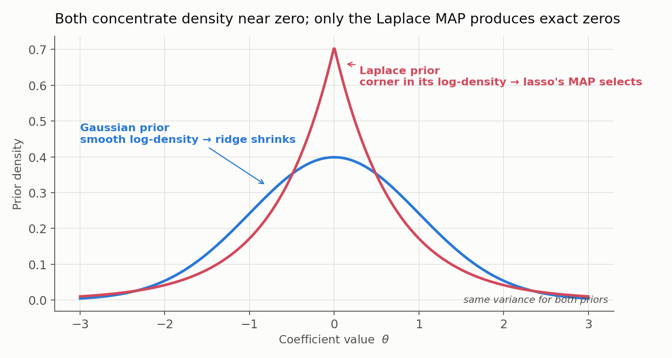
The figure shows both prior densities at equal variance; both peak at zero. The difference that matters lives one derivative down, in the negative log-density - which is exactly the penalty. The Gaussian’s negative log-density is $\theta^2/2\tau^2$: smooth, with zero slope at the origin, so its pull fades as a coefficient approaches zero and nothing ever pushes an estimate the last millimeter to exactly zero. The Laplace’s negative log-density is $\vert\theta\vert/b$: it has a corner at the origin with a nonzero one-sided slope, a constant pull that does not fade. At the MAP optimum that corner produces soft-thresholding: weak coefficients get dragged to exactly zero and pinned there. Shrinkage versus selection is a statement about the penalty’s slope at the origin.

The classic geometric picture says the same thing in the loss landscape. Writing the penalized problems in constrained form, ridge confines $\theta$ to a disk and lasso to a diamond, and the fit is where the loss contours first touch the constraint set:

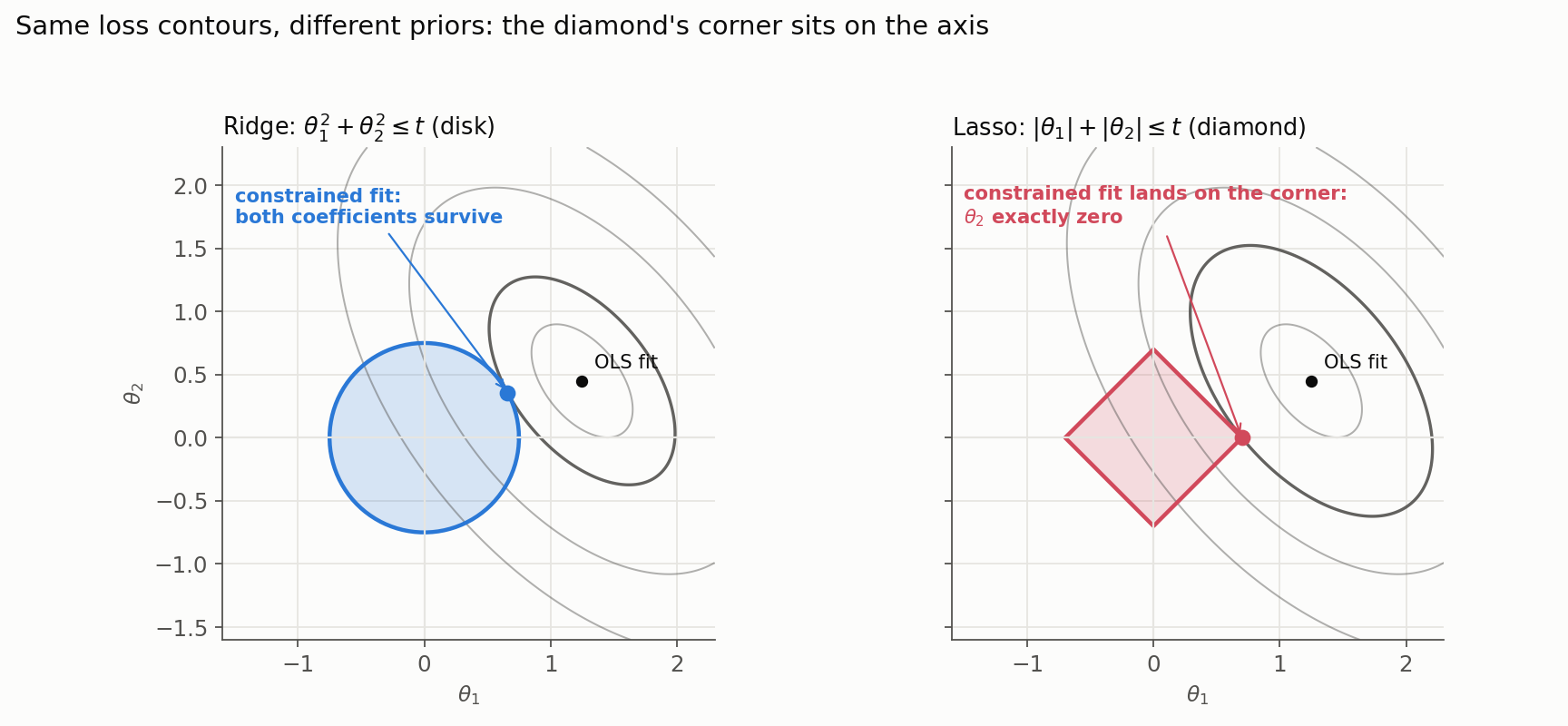
A disk has no special points: the touch can happen anywhere, so both coefficients survive (smaller, but alive). A diamond has corners, the corners sit on the axes, and corners stick out furthest toward the contours, so the touch lands there disproportionately often. A corner on an axis is precisely “one coefficient exactly zero.”

The nuance almost every summary garbles. Lasso is the MAP estimate under a Laplace prior; it is not “the Bayesian answer.” The full posterior under a Laplace prior is not sparse: the posterior probability that any coefficient equals exactly zero is zero (it is a continuous distribution), the posterior mean is essentially never exactly zero, and the Laplace prior is not Gaussian-conjugate, so this posterior lacks the Gaussian closed form. Sparsity is a property of the peak of that posterior, not of the belief as a whole. So “lasso = Bayesian variable selection” oversells it: a fully Bayesian treatment of sparsity needs priors with genuine mass at zero (spike-and-slab and relatives), which buy honesty about selection uncertainty at a real computational price. Lasso is best understood as a superb frequentist estimator whose form is explained by a Bayesian identity.

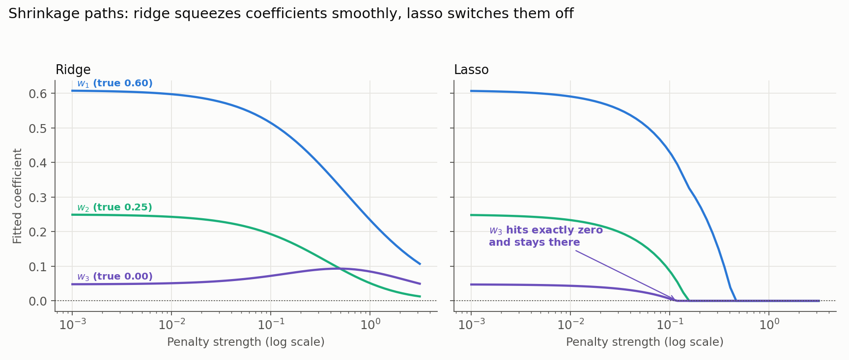
Watching the blade work. Sparsity needs more than one feature to be visible, so we simulate a three-feature problem and fit both estimators. The full recipe, so the numbers are reproducible: 40 observations; features drawn independently from $\mathcal{N}(0,1)$ (uncorrelated by design, though finite samples leave incidental correlations); outcome $y = Xw + \varepsilon$ with true weights $(0.60, 0.25, 0.00)$ and noise standard deviation $0.3$; a fixed seed; no intercept; scikit-learn’s Ridge and Lasso with default centering. One caveat before reading the table’s knob: the two estimators normalize their objectives differently - Ridge minimizes $\lVert y - Xw \rVert^2 + \alpha_R \lVert w \rVert^2$ while Lasso minimizes $\frac{1}{2n}\lVert y - Xw \rVert^2 + \alpha_L \lVert w \rVert_1$ - and an L2 and an L1 penalty are not unit-comparable in any case. We pass the ridge solver $n \alpha$ to put both on a roughly per-sample footing, but the $\alpha$ values below are best read as illustrative solver parameters, one column at a time, not as matched strengths:

Penalty strength	Ridge coefficients	Lasso coefficients
Light ($\alpha = 0.05$)	$(0.557,\, 0.218,\, 0.062)$	$(0.519,\, 0.168,\, 0.027)$
Medium ($\alpha = 0.1$)	$(0.514,\, 0.193,\, 0.072)$	$(0.430,\, 0.086,\, 0.006)$
Heavy ($\alpha = 0.2$)	$(0.448,\, 0.155,\, 0.085)$	$(0.276,\, 0.000,\, 0.000)$

Ridge generally does not set coefficients exactly to zero; it carries the useless $w_3$, shrunken, indefinitely - and note in the paths below that with finite data an individual ridge coefficient need not even shrink monotonically ($w_3$ drifts upward before falling, a side effect of the incidental correlations among features). Lasso drives $w_3$ to exactly zero, and at heavy penalty kills the genuinely useful but weak $w_2$ as well: selection is a blade, and it does not only cut where we would like.

---

5. A Posterior by Hand

Time for real numbers, small enough to check every step. We observe six points, with a standardized feature $z$ and outcome $y$:

$z$	$-1.2$	$-0.7$	$-0.2$	$0.3$	$0.8$	$1.0$
$y$	$0.16$	$0.27$	$0.47$	$0.55$	$0.78$	$0.82$

The features are $x_i = (1, z_i)^\top$ and the noise scale is known, $\sigma = 0.10$. Following the practical convention from section 3, we leave the intercept unpenalized (a flat prior: the $\tau \to \infty$ limit, contributing zero to the penalty) and put the Gaussian prior only on the slope, with $\lambda = \sigma^2/\tau^2 = 1$. The penalty is then a matrix with one active entry:

\[\Lambda = \begin{bmatrix} 0 & 0\\ 0 & 1 \end{bmatrix}\]

Unknown to the fit, the data was generated from $y = 0.5 + 0.3z$ plus noise.

Build the two memory objects. The feature sums are $\sum z_i = 0$ (by design, to keep the arithmetic transparent) and $\sum z_i^2 = 3.70$, so:

\[A = \Lambda + X^\top X = \begin{bmatrix} 6 & 0\\ 0 & 4.70 \end{bmatrix}, \qquad b = X^\top y = \begin{bmatrix} 3.05\\ 1.134 \end{bmatrix}\]

Because $A$ is diagonal, the inversion is mental arithmetic, and the whole posterior follows:

\[\hat{\theta} = A^{-1} b = \begin{bmatrix} 3.05 / 6\\ 1.134 / 4.70 \end{bmatrix} = \begin{bmatrix} 0.508\\ 0.241 \end{bmatrix}, \qquad \Sigma_{\text{post}} = \sigma^2 A^{-1} = \begin{bmatrix} 0.00167 & 0\\ 0 & 0.00213 \end{bmatrix}\]

Three readings of this result:

• Shrinkage is visible, and selective. The OLS fit on the same data is $(0.508, 0.307)$. The posterior intercept is identical to OLS - a flat prior adds nothing, and with $\sum z_i = 0$ the intercept decouples cleanly - while the slope shrinks from $0.307$ to $0.241$, pulled toward zero by its prior. The convention is visible in the arithmetic: only what carries a prior gets shrunk.
• The posterior has widths, not just a center. The coefficient standard deviations are $\sqrt{0.00167} \approx 0.041$ for the intercept and $\sqrt{0.00213} \approx 0.046$ for the slope. A 95% credible interval for the slope is $0.241 \pm 1.96 \cdot 0.046 = [0.151,\, 0.332]$, which comfortably contains the true 0.3. The interpretation is worth stating exactly: conditional on this model and this data, the posterior assigns 95% probability to that interval.
• More data where it matters would tighten exactly the right entries. The slope variance divides by $\lambda + \sum z_i^2$: spread-out observations (large $\vert z \vert$) are what buy slope certainty. The matrix $A$ is quietly keeping “where did the data sit” books, and the posterior’s widths read them back.

---

6. The Predictive Distribution: What the Posterior Is For

The posterior over coefficients is a means to an end; what we usually want is a prediction for a new input, with its uncertainty. The Bayesian answer averages predictions over every plausible line, and for the Gaussian model it comes out in closed form. For a new input $x$:

\[y_{\text{new}} \mid x, \text{data} \;\sim\; \mathcal{N}\!\left( x^\top \hat{\theta}, \;\; \sigma^2 + x^\top \Sigma_{\text{post}} \, x \right)\]

The predictive variance has two parts with different characters, and they combine inside the variance ($\sigma^2 + x^\top \Sigma_{\text{post}}\, x$), not by adding interval widths. The $\sigma^2$ term is noise floor: irreducible scatter that no amount of data removes. The $x^\top \Sigma_{\text{post}}\, x$ term is remaining ignorance about the line itself, and it depends on where we predict: small amid the training data, growing as we extrapolate. On our worked example, the predictive standard deviation is $0.108$ at $z = 0$ but $0.126$ out at $z = 1.4$, and the widening is visible:

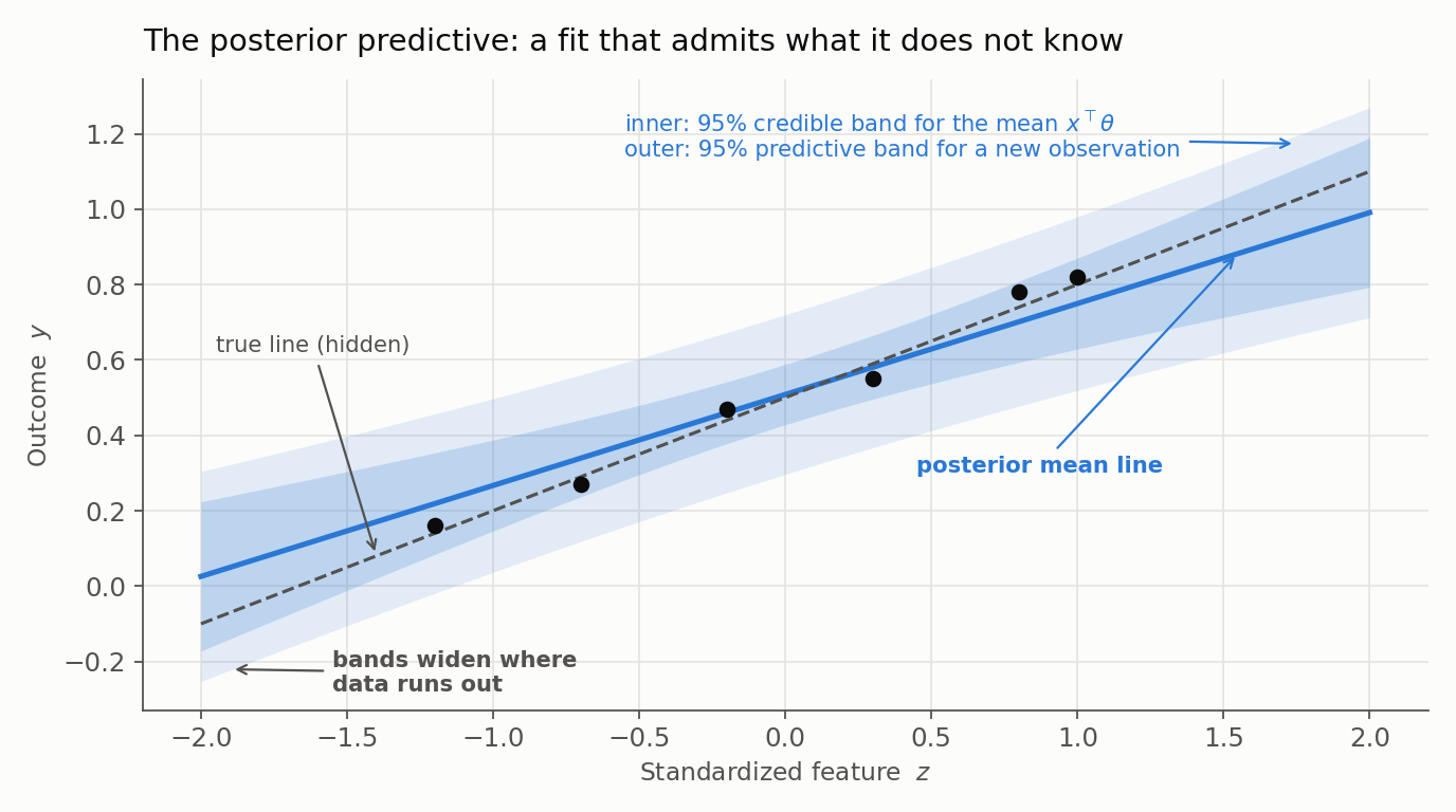
The two bands are pointwise 95% intervals with distinct meanings: the inner one is a credible band for the latent mean $x^\top\theta$ (where the true line plausibly runs), the outer a posterior predictive band for a new observation (where the next data point plausibly lands). This location-dependent uncertainty is the piece worth remembering: any system that must know where its model can be trusted reads the answer off exactly this quadratic form.

Two qualifications keep the bands honest. First, this is model-based uncertainty: the bands are trustworthy only to the extent that the linear mean, the Gaussian constant-variance noise, the prior, and the feature representation are adequate. They widen with leverage, but they cannot warn us that the model class itself is wrong - a nonlinear truth, an omitted variable, or a distribution shift can sit squarely inside a confident band. Second, the clean Normal form above assumes $\sigma$ is known; when $\sigma^2$ is unknown and integrated out under the standard conjugate prior, the posterior predictive becomes Student-$t$, its heavier tails reflecting the extra uncertainty about the noise scale.

---

7. Beyond MAP: When the Peak Misleads

If MAP, posterior mean, and ridge coincide here, why carry the full posterior at all? Three reasons, in increasing order of consequence:

• Intervals are part of the answer. The credible interval $[0.151, 0.332]$ for our slope is a statement of belief we can act on; a bare 0.241 is not. Any downstream decision that depends on how sure we are (bet sizing, exploration, go/no-go calls) needs the width, not the peak.
• The coincidence is a Gaussian special case. Peak equals mean here because the posterior is Gaussian. Under a Laplace prior (section 4), or any skewed posterior, MAP and mean diverge, and the peak can sit far from where the probability mass actually lives. Summarizing a skewed belief by its peak is how the lasso-is-Bayesian confusion starts.
• Downstream algorithms may need the whole distribution. Adaptive systems that balance learning against earning (posterior-sampling methods in sequential experimentation) do not want a point estimate; they sample coefficient vectors from this exact posterior to drive exploration. Collapse the posterior and such an algorithm stops working.

Left deliberately outside this post: treating $\sigma$ and $\tau$ as unknowns with their own priors (full hierarchies), or estimating them from the data’s marginal likelihood (empirical Bayes), and the spike-and-slab family for genuinely Bayesian sparsity. Those extend the same machinery rather than replacing it.

---

Where This Sits

One identity organized this whole post: penalty = negative log-prior. Ridge and lasso stop being arbitrary tricks and become two beliefs about coefficients: the Gaussian’s “small, smoothly” and the Laplace’s “mostly zero, occasionally large”. The Gaussian branch, thanks to conjugacy, yields a closed-form posterior whose predictive bands retain the uncertainty that a MAP estimate alone discards. And the construction generalizes: swap the Gaussian likelihood for a Bernoulli or Poisson one and the same prior-plus-likelihood recipe keeps going, just without the closed forms.

Happy fitting - and may every penalty in our loss functions henceforth introduce itself honestly, as the prior it always was.

---

Resources

• Bayesian Linear Regression: Data Science Concepts - a friendly video walkthrough of the prior-to-posterior mechanics this post derives.
• Hoerl, A. E. and Kennard, R. W. (1970), “Ridge Regression: Biased Estimation for Nonorthogonal Problems”, Technometrics, 12(1), 55-67 - the original ridge paper.
• Tibshirani, R. (1996), “Regression Shrinkage and Selection via the Lasso”, Journal of the Royal Statistical Society: Series B, 58(1), 267-288 - the original lasso paper.
• Park, T. and Casella, G. (2008), “The Bayesian Lasso”, Journal of the American Statistical Association, 103(482), 681-686 - the fully Bayesian treatment of the Laplace prior, and the natural next step from section 4’s nuance.
• scikit-learn’s linear-model documentation - the objective conventions behind section 4’s solver parameters.