Probability Distribution: Beta
The Beta distribution models a proportion or probability on [0,1]: how its two shape parameters bend the curve, its role as the Binomial's conjugate prior, a worked Bayesian update, and when it fits.
The Question It Answers
How is a proportion, or a probability, some number between 0 and 1, distributed? The Beta distribution lives entirely on $[0, 1]$, which makes it the natural language for uncertain rates: a click-through rate, a conversion probability, a defect fraction. Its headline role is as the conjugate prior for the Binomial: start with a Beta belief about a success probability, observe some successes and failures, and the updated belief is again a Beta.
| Field | Content |
|---|---|
| Type | Continuous |
| Random variable | $X$ = a proportion or probability |
| Support | $0 \le X \le 1$ |
| Parameters | $\alpha > 0$, $\beta > 0$ (shape parameters; loosely “prior successes” and “prior failures”) |
| Mean | $\alpha/(\alpha + \beta)$ |
| Variance | $\dfrac{\alpha\beta}{(\alpha + \beta)^2 (\alpha + \beta + 1)}$ |
| Signature | Flexible shapes on $[0, 1]$; conjugate to the Binomial |
Shape Before Formula
The two parameters pull mass toward the two ends. With $\alpha = \beta$ the curve is symmetric about $0.5$; raising both sharpens the peak (more certainty), while lowering both below 1 hollows it into a U that piles mass at 0 and 1. Making $\alpha > \beta$ tilts it toward 1, and $\alpha < \beta$ toward 0. The flat Uniform is exactly Beta$(1, 1)$: total ignorance across $[0, 1]$.
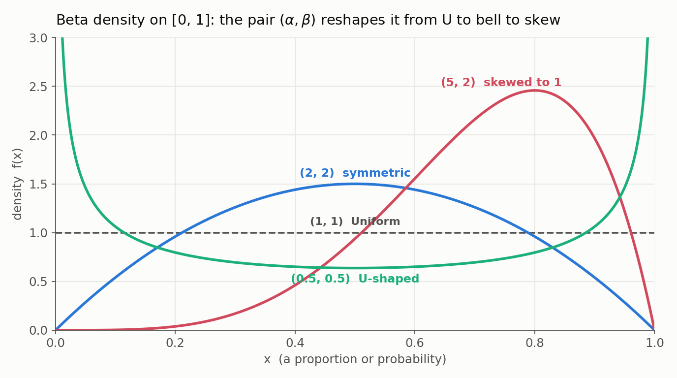
The normalizer is the beta function $B(\alpha, \beta) = \int_0^1 t^{\alpha - 1}(1 - t)^{\beta - 1}\,dt = \Gamma(\alpha)\Gamma(\beta)/\Gamma(\alpha + \beta)$, which is exactly what makes the area integrate to one.
A Worked Example: Updating a Click-Through Rate
Setup. We want the click-through rate $p$ of a new ad. Before any data we hold a weak, symmetric prior $p \sim \text{Beta}(2, 2)$: centered at $0.5$ (mean $\alpha/(\alpha + \beta) = 0.5$) but broad. We then show the ad 10 times and see 8 clicks and 2 misses.
Conjugacy makes the update arithmetic rather than calculus: a Beta$(\alpha, \beta)$ prior combined with $s$ successes and $f$ failures becomes a Beta$(\alpha + s, \beta + f)$ posterior. Here that is
\[p \mid \text{data} \sim \text{Beta}(2 + 8,\; 2 + 2) = \text{Beta}(10, 4).\]- Posterior mean: $10/(10 + 4) = 0.714$, pulled up from the prior’s $0.5$ by the data.
- Is the rate above one-half? $P(p > 0.5) = 1 - F(0.5) \approx 0.954$: strong, though not decisive, evidence.
- 95% credible interval: the 2.5th to 97.5th posterior percentiles run from about $0.46$ to $0.91$, still wide after only 10 trials.
Here $F$ is the Beta CDF, the regularized incomplete beta function, evaluated numerically.
Concentration: How Much the Data Has Spoken
The sum $\alpha + \beta$ acts as a concentration, a pseudo-sample-size: the larger it is, the tighter the distribution around its mean. Our posterior’s $\alpha + \beta = 14$ encodes “as if we had seen about 14 trials.” The same mean $0.714$ from a Beta$(100, 40)$ would be far narrower. This is why a Beta$(1, 1)$ prior (concentration 2) is quickly overwhelmed by data, while a Beta$(50, 50)$ prior takes real evidence to move: the prior’s concentration is literally how many pseudo-observations it is worth.
When It Fits, and When It Fails
| Assumes | The quantity is a single proportion confined to $[0, 1]$; the two shape parameters capture where its mass sits |
| Common violation | Quantities that can exceed 1 or are unbounded; a spike of exact 0s or 1s (zero-or-one inflation) a smooth density cannot represent; reading $\alpha, \beta$ as exact event counts when they are only shape parameters |
| Closest relatives | Binomial (the conjugate likelihood); Uniform (the Beta$(1, 1)$ case); Gamma (if $U \sim$ Gamma$(\alpha)$ and $V \sim$ Gamma$(\beta)$ are independent, then $U/(U + V) \sim$ Beta$(\alpha, \beta)$); Dirichlet (its multivariate generalization to several proportions) |
Modeling a conversion rate as Beta says the rate is one fixed number we are uncertain about, not a mixture of distinct segments each with its own rate. When the traffic is really two populations, a single Beta hides the split.
A Minimal Code Check
1
2
3
4
5
6
7
from scipy.stats import beta

post = beta(10, 4)          # Beta(2,2) prior + 8 successes, 2 failures
post.mean()                 # 0.714
1 - post.cdf(0.5)           # P(p > 0.5)         -> 0.954
post.ppf([0.025, 0.975])    # 95% credible band  -> [0.46, 0.91]
beta(1, 1).pdf(0.3)         # the Uniform is Beta(1,1) -> 1.0
SciPy’s beta(a, b) takes the shape parameters directly. Note the name clash: the beta distribution and the beta function $B(\alpha, \beta)$ are different objects; the distribution uses the function only as its normalizer.
Appendix: Deriving the Mean and Variance
Every moment of the Beta reduces to a ratio of beta functions, using $\int_0^1 x^{\alpha - 1}(1 - x)^{\beta - 1}\,dx = B(\alpha, \beta)$, the recurrence $B(\alpha, \beta) = \Gamma(\alpha)\Gamma(\beta)/\Gamma(\alpha + \beta)$, and $\Gamma(z + 1) = z\,\Gamma(z)$.
The Mean
Multiplying the density by $x$ raises the first exponent by one:
\[E[X] = \frac{1}{B(\alpha, \beta)}\int_0^1 x^{\alpha}(1 - x)^{\beta - 1}\,dx = \frac{B(\alpha + 1, \beta)}{B(\alpha, \beta)}.\]Expanding both beta functions in gamma functions, everything cancels except
\[\frac{B(\alpha + 1, \beta)}{B(\alpha, \beta)} = \frac{\Gamma(\alpha + 1)}{\Gamma(\alpha)}\cdot\frac{\Gamma(\alpha + \beta)}{\Gamma(\alpha + \beta + 1)} = \frac{\alpha}{\alpha + \beta}.\]The Variance
The same step with $x^2$ gives the second moment as $B(\alpha + 2, \beta)/B(\alpha, \beta)$:
\[E[X^2] = \frac{\alpha(\alpha + 1)}{(\alpha + \beta)(\alpha + \beta + 1)}.\]Subtracting the squared mean and combining over a common denominator,
\[\text{Var}(X) = \frac{\alpha(\alpha + 1)}{(\alpha + \beta)(\alpha + \beta + 1)} - \left(\frac{\alpha}{\alpha + \beta}\right)^2 = \frac{\alpha\beta}{(\alpha + \beta)^2 (\alpha + \beta + 1)}.\]The $(\alpha + \beta + 1)$ in the denominator is the concentration at work: holding the mean fixed, a larger $\alpha + \beta$ shrinks the variance.
Where this sits in the series. Previous concept: Gamma (waiting time for the $k$-th event). This is the final distribution; return to the series overview for the full map. Closest cousins: Binomial (the conjugate likelihood) and the Uniform (its flat $\alpha = \beta = 1$ case).