Probability Distribution: Poisson
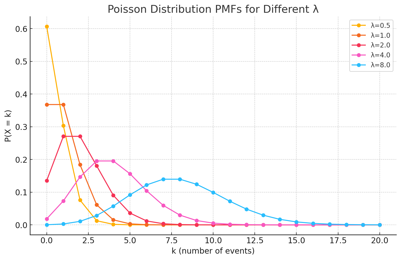
The Poisson distribution models the probability of a given number of events happening in a fixed interval of time or space, assuming these events occur with a known constant mean rate and independently of the time since the last event. The key parameter is lambda ($\lambda$), which represents the average number of events in that interval.
Probability Mass Function (PMF)
The PMF gives the probability of observing exactly k events in an interval.
\[P(X=k) = \frac{\lambda^k e^{-\lambda}}{k!}\]Where:
- k is the number of occurrences (k = 0, 1, 2, …).
- $\lambda$ is the average number of occurrences per interval.
- e is Euler’s number (approximately 2.71828).
Derivations
For a Poisson distribution, both the mean and the variance are equal to $\lambda$.
Derivation of the Mean (E[X])
The mean is the expected value, calculated by summing $k * P(X=k)$ for all possible values of $k$.
Definition of Expected Value:
\[E[X] = \sum_{k=0}^{\infty} k \cdot P(X=k) = \sum_{k=0}^{\infty} k \cdot \frac{\lambda^k e^{-\lambda}}{k!}\]Simplify the Sum: The term for $k=0$ is 0, so we can start the sum from $k=1$. We then simplify $k/k!$ to $1/(k-1)!$.
\[E[X] = e^{-\lambda} \sum_{k=1}^{\infty} k \cdot \frac{\lambda^k}{k!} = e^{-\lambda} \sum_{k=1}^{\infty} \frac{\lambda^k}{(k-1)!}\]Factor out $\lambda$ and Re-index: We factor out $\lambda$ to make the exponents match the factorial term. Let $n = k-1$.
\[E[X] = e^{-\lambda} \lambda \sum_{k=1}^{\infty} \frac{\lambda^{k-1}}{(k-1)!} = e^{-\lambda} \lambda \sum_{n=0}^{\infty} \frac{\lambda^{n}}{n!}\]Use the Taylor Series for $e^\lambda$: The sum $\sum_{n=0}^{\infty} \frac{\lambda^{n}}{n!}$ is the Taylor series expansion for $e^\lambda$.
\[E[X] = e^{-\lambda} \lambda (e^{\lambda})\]Final Result:
\[E[X] = \lambda\]
Derivation of the Variance (Var(X))
We use the formula $Var(X) = E[X^2] - (E[X])^2$. The trick is to find $E[X(X-1)]$ first.
Find E[X(X-1)]:
\[E[X(X-1)] = \sum_{k=0}^{\infty} k(k-1) \cdot \frac{\lambda^k e^{-\lambda}}{k!} = e^{-\lambda} \sum_{k=2}^{\infty} \frac{\lambda^k}{(k-2)!}\]The terms for $k=0$ and $k=1$ are zero. We factor out $\lambda^2$ and re-index with $n = k-2$.
\[E[X(X-1)] = e^{-\lambda} \lambda^2 \sum_{k=2}^{\infty} \frac{\lambda^{k-2}}{(k-2)!} = e^{-\lambda} \lambda^2 \sum_{n=0}^{\infty} \frac{\lambda^{n}}{n!} = e^{-\lambda} \lambda^2 (e^{\lambda}) = \lambda^2\]Calculate E[X²]: We know $E[X(X-1)] = E[X^2] - E[X]$. Therefore:
\[E[X^2] = E[X(X-1)] + E[X] = \lambda^2 + \lambda\]Calculate the Variance:
\[Var(X) = E[X^2] - (E[X])^2 = (\lambda^2 + \lambda) - (\lambda)^2\]Final Result:
\[Var(X) = \lambda\]
Practical Scenarios
Scenario 1: Call Center Traffic
Situation: A customer support call center receives an average of 5 calls per hour ($\lambda = 5$). We want to know the probability of receiving exactly 2 calls in the next hour.
Derivation: We use the PMF with $k=2$ and $\lambda=5$.
\[P(X=2) = \frac{5^2 e^{-5}}{2!} = \frac{25 \cdot e^{-5}}{2}\]Using $e^{-5} \approx 0.006738$:
\[P(X=2) \approx \frac{25 \cdot 0.006738}{2} \approx 0.084\]There is approximately an 8.4% chance of receiving exactly 2 calls in the next hour.
Scenario 2: Website Errors
Situation: A web server experiences an average of 3 bugs per day ($\lambda = 3$). We want to find the probability of experiencing no bugs at all on a given day.
Derivation: We use the PMF with $k=0$ and $\lambda=3$.
\[P(X=0) = \frac{3^0 e^{-3}}{0!}\]Since $3^0 = 1$ and $0! = 1$:
\[P(X=0) = e^{-3} \approx 0.0498\]There is approximately a 5% chance that the server will have a bug-free day.
Estimating MTTF
You can estimate Mean Time To Failure (MTTF) in a supply chain using a Poisson process. The relationship between the two is a fundamental concept in reliability engineering.
The connection works like this: If the number of failures in a given time period follows a Poisson distribution (describing the count of events), then the time between those failures follows an Exponential distribution. The mean of this exponential distribution is the MTTF.
The Conceptual Link: Poisson vs. Exponential
Poisson Process: Models the number of failures occurring in a fixed interval. It’s defined by the failure rate, λ (lambda), which is the average number of failures per unit of time (e.g., failures per month).
MTTF (from the Exponential Distribution): Models the time between individual failures. It is the reciprocal of the Poisson failure rate.
\[MTTF = \frac{1}{\lambda}\]
Example: Estimating MTTF for a Warehouse Sorting Machine
Let’s say you’re a manager at a distribution center, and you want to estimate the MTTF for a critical automated sorting machine to better plan your maintenance schedule.
Step 1: Gather Historical Data
You look at the maintenance logs for the machine over the last 36 months (3 years). In that time, the machine experienced 12 critical failures that halted operations.
Step 2: Calculate the Failure Rate (λ)
First, you calculate the average number of failures per unit of time. It’s common to use a year as the unit.
- Total Failures: 12
- Total Time: 3 years
Failure Rate (λ):
\[\lambda = \frac{\text{Total Failures}}{\text{Total Time}} = \frac{12 \text{ failures}}{3 \text{ years}} = 4 \text{ failures per year}\]This means the machine fails at an average rate of 4 times per year.
Step 3: Estimate the MTTF
Now, you use the core relationship to find the average time between each of those failures.
MTTF Calculation:
\[MTTF = \frac{1}{\lambda} = \frac{1}{4 \text{ failures/year}} = 0.25 \text{ years}\]
Step 4: Interpret the Result
To make this more practical for maintenance planning, you can convert the MTTF into a more intuitive unit, like months.
Interpretation:
\[0.25 \text{ years} \times 12 \text{ months/year} = 3 \text{ months}\]
Conclusion: Based on the historical data, you can estimate that the Mean Time To Failure (MTTF) for this sorting machine is 3 months. This insight allows you to schedule preventive maintenance checks more effectively, perhaps every 2 or 2.5 months, to minimize unexpected downtime in your supply chain.