Probability Distribution: Gamma
The Gamma distribution models the waiting time until the k-th constant-rate event: its shape and rate parameters, the Poisson-tail reading of its CDF, how it generalizes the Exponential, and when it fails.
The Question It Answers
How long until the $k$-th event, when events arrive at a constant average rate? Where the Exponential times the wait to the next event, the Gamma times the wait to the $k$-th. Add up $k$ independent Exponential waits, each at rate $\lambda$, and their total is Gamma-distributed. It doubles as a flexible model for any positive, right-skewed quantity: rainfall totals, insurance claim sizes, task durations.
| Field | Content |
|---|---|
| Type | Continuous |
| Random variable | $X$ = waiting time until the $k$-th event (or any positive magnitude) |
| Support | $X > 0$ |
| Parameters | shape $k > 0$ (dimensionless); rate $\lambda > 0$ (inverse time), with scale $\theta = 1/\lambda$ |
| Mean | $k/\lambda = k\theta$ |
| Variance | $k/\lambda^2 = k\theta^2$ |
| Signature | Sum of $k$ Exponential waits (integer $k$); skewness $2/\sqrt{k}$ shrinks as $k$ grows |
Shape Before Formula
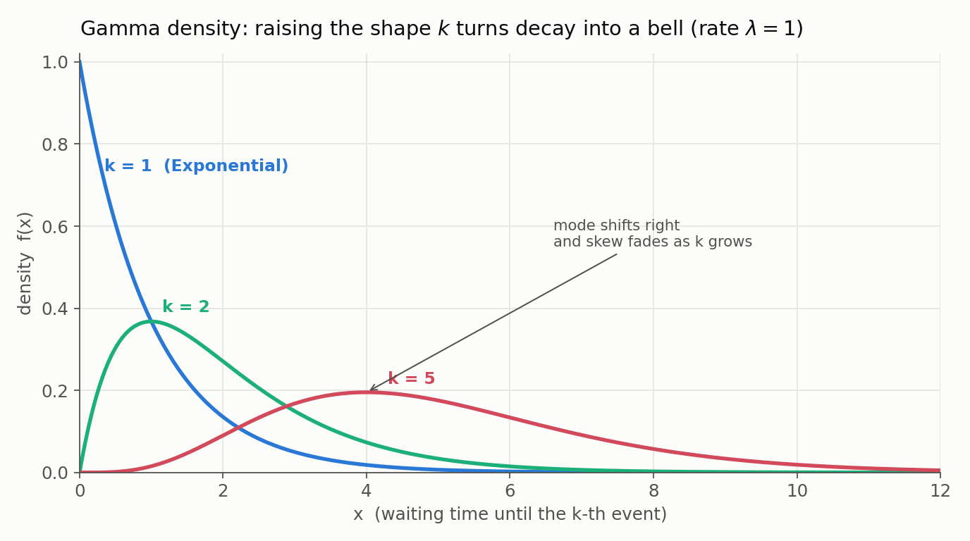
The shape parameter $k$ carries the story. At $k = 1$ the Gamma is the Exponential, decaying from its peak at zero. For $k > 1$ the density starts at zero, climbs to a mode at $(k-1)/\lambda$, and trails off in a right skew that fades as $k$ rises; by large $k$ it looks Normal, a sum of many independent waits courtesy of the central limit theorem.
The normalizer is the gamma function $\Gamma(k) = \int_0^\infty t^{k-1} e^{-t}\,dt$, which extends the factorial: $\Gamma(k) = (k-1)!$ for integer $k$. When $k$ is a positive integer the distribution is also called the Erlang, and only then does the “time of the $k$-th arrival” reading apply literally, even though the density is well defined for any real $k > 0$.
A Worked Example: Time to the Third Call
Setup. Calls arrive at $\lambda = 5$ per hour (Poisson arrivals). The wait until the third call is $X \sim \text{Gamma}(k = 3, \lambda = 5)$, with mean $k/\lambda = 3/5$ hour $= 36$ minutes.
For integer $k$ the Gamma CDF reads cleanly through the Poisson: the $k$-th event has arrived by time $t$ exactly when at least $k$ events have occurred in $[0, t]$, so
\[P(X \le t) = P\big(N(t) \ge k\big), \qquad N(t) \sim \text{Poisson}(\lambda t).\]- Third call within the hour ($t = 1$, so $\lambda t = 5$): $P(X \le 1) = P(N \ge 3) = 1 - e^{-5}(1 + 5 + 12.5) \approx 0.875$.
- Within half an hour ($t = 0.5$, so $\lambda t = 2.5$): $P(X \le 0.5) = 1 - e^{-2.5}(1 + 2.5 + 3.125) \approx 0.456$.
- Between 30 and 60 minutes: $0.875 - 0.456 \approx 0.419$.
Beyond the Density: Three Centers and the CDF
Because the Gamma is right-skewed for finite $k$, its three centers separate in a fixed order: mode $(k-1)/\lambda <$ median $<$ mean $k/\lambda$. For the example that is mode $= 24$ min, median $\approx 32$ min, mean $= 36$ min, the long right tail dragging the mean above the median. The general CDF is the regularized lower incomplete gamma function $P(X \le t) = \gamma(k, \lambda t)/\Gamma(k)$, which for non-integer $k$ has no elementary closed form and is evaluated numerically.
Additivity, and the Exponential Family
Two facts make the Gamma more than “a skewed positive density.” First, it is built from Exponentials: summing $k$ independent Exponential($\lambda$) waits yields exactly Gamma($k, \lambda$), which is why integer $k$ reads as the time of the $k$-th arrival. Second, it is additive at a fixed rate: independent Gamma($k_1, \lambda$) and Gamma($k_2, \lambda$) variables sum to Gamma($k_1 + k_2, \lambda$), the continuous echo of adding independent Poisson counts. Two familiar distributions are Gamma in disguise: the Exponential is the $k = 1$ case, and the chi-squared with $\nu$ degrees of freedom is Gamma($k = \nu/2$, $\lambda = 1/2$), which is why sums of squared Normals turn up Gamma-shaped.
When It Fits, and When It Fails
| Assumes | For the arrival reading: $k$ independent stages, each a constant-rate memoryless wait at the same rate $\lambda$ |
| Common violation | Stages with different rates (the sum is then a general phase-type law, not Gamma); a non-monotone hazard; tails heavier than Gamma’s exponential decay |
| Closest relatives | Exponential ($k = 1$); Erlang (integer $k$); chi-squared ($k = \nu/2$, $\lambda = 1/2$); Normal (large-$k$ limit); Weibull and Log-Normal (other positive, skewed models) |
Fitting task durations as Gamma assumes each hidden stage clears at the same constant rate: a claim about the mechanism, not just about the histogram’s shape.
A Minimal Code Check
1
2
3
4
5
6
7
8
from scipy.stats import gamma, poisson

k, lam = 3, 5.0                    # 3rd call; scipy uses shape a = k, scale = 1/lam
X = gamma(a=k, scale=1/lam)
X.mean(), X.var()                  # (0.6 h, 0.12) = (k/lam, k/lam**2)
X.cdf(1.0)                         # 3rd call within 1 h      -> 0.875
1 - poisson.cdf(k - 1, lam * 1.0)  # same value via the Poisson tail -> 0.875
X.ppf(0.5)                         # median wait (h)          -> ~0.535 (32 min)
As with the Exponential, scipy.stats.gamma takes scale = 1/lambda, not a rate. The agreement between gamma.cdf and the Poisson tail is the arrival-count identity made concrete.
Appendix: Deriving the Mean and Variance
Both moments come from a single fact, that the density integrates to one, which is the gamma-function identity $\int_0^\infty x^{k-1} e^{-\lambda x}\,dx = \Gamma(k)/\lambda^k$.
The Mean
Multiplying the density by $x$ raises the power by one:
\[E[X] = \int_0^\infty x\,\frac{\lambda^k}{\Gamma(k)}\, x^{k-1} e^{-\lambda x}\,dx = \frac{\lambda^k}{\Gamma(k)}\int_0^\infty x^{k} e^{-\lambda x}\,dx.\]The integral is $\Gamma(k+1)/\lambda^{k+1}$, and $\Gamma(k+1) = k\,\Gamma(k)$, so
\[E[X] = \frac{\lambda^k}{\Gamma(k)}\cdot\frac{k\,\Gamma(k)}{\lambda^{k+1}} = \frac{k}{\lambda}.\]The Variance
The same identity with one more power of $x$ gives the second moment, using $\Gamma(k+2) = (k+1)\,k\,\Gamma(k)$:
\[E[X^2] = \frac{\lambda^k}{\Gamma(k)}\int_0^\infty x^{k+1} e^{-\lambda x}\,dx = \frac{\lambda^k}{\Gamma(k)}\cdot\frac{\Gamma(k+2)}{\lambda^{k+2}} = \frac{k(k+1)}{\lambda^2}.\]Therefore
\[\text{Var}(X) = E[X^2] - (E[X])^2 = \frac{k(k+1)}{\lambda^2} - \frac{k^2}{\lambda^2} = \frac{k}{\lambda^2}.\]The integer-$k$ reading makes both results immediate: $X$ is a sum of $k$ independent Exponential($\lambda$) waits, each with mean $1/\lambda$ and variance $1/\lambda^2$, so linearity and independence give $k/\lambda$ and $k/\lambda^2$ directly.
Where this sits in the series. Previous concept: Laplace. Next concept: Beta (a distribution over proportions). Closest cousins: Exponential (the $k = 1$ case) and Poisson (the arrival-count dual). Series overview.