Linear Regression, Part 3: Evaluation, Interpretation, and Extensions

Linear Regression series: Part 1: OLS Foundations · Part 2: Multicollinearity and Regularization · Part 3: Evaluation, Interpretation, and Extensions

Part 1 established the OLS machinery, while Part 2 handled multicollinearity and regularization. With a fitted and stable model in hand, the remaining challenge is using it responsibly.

This final part covers evaluation, robustness, and interpretation. We will examine $R^2$, outliers, coefficient meaning, and feature importance before widening the framework from vanilla linear regression to Generalized Linear Models (GLMs).

---

1. Evaluating a Regression Model with $R^2$

Let’s break down the formulation of R-squared ($R^2$) and, most importantly, how to interpret what it tells us about our regression model.

Conceptual Goal of R-squared

At its core, R-squared measures the proportion of the variance in the dependent variable that is predictable from the independent variable(s).

In simpler terms, it tells us what percentage of the “movement” in the target variable (e.g., house prices) can be explained by the features in our model (e.g., square footage, number of bedrooms).

The Formulation of R-squared

To understand the formula, we first need to understand two key components:

1. Total Sum of Squares (SST or SSTO): This represents the total variation in the dependent variable. It’s calculated by summing the squared differences between each actual data point ($y_i$) and the mean of all data points ($\bar{y}$). Think of this as the error we would have if we used a very simple baseline model that just predicts the average value for every data point.

   \[SST = \sum_{i=1}^{n} (y_i - \bar{y})^2\]

2. Sum of Squared Residuals (SSR or SSE): This represents the variation that is left unexplained by our model after it has been trained. It’s the sum of the squared differences between each actual data point ($y_i$) and the value predicted by our model ($\hat{y}_i$). This is our model’s error.

   \[SSR = \sum_{i=1}^{n} (y_i - \hat{y}_i)^2\]

   (A naming caution: textbooks use SSR inconsistently - some mean the residual sum of squares, as we do here, while others use it for the regression sum of squares and write the residual one as RSS or SSE. Check the convention before comparing formulas across sources.)

Now, the R-squared formula brings these two components together:

\[R^2 = 1 - \frac{SSR}{SST}\]

Breaking Down the Formula’s Logic:

• The fraction $\frac{SSR}{SST}$ represents the proportion of the total variance that is not explained by our model. It’s the fraction of the total error that remains in our model’s residuals.
• By subtracting this fraction from 1, we get the proportion of the total variance that is explained by our model.

How to Interpret the R-squared Value

For an in-sample OLS fit that includes an intercept, R-squared lands between 0 and 1 (0% and 100%) - the qualifier matters, as the caveats below explain. Here is how to interpret that range:

• An R-squared of 1 (or 100%):
  • Interpretation: The model explains all the variability of the response data around its mean.
  • Meaning: The predictions ($\hat{y}_i$) are exactly equal to the actual values ($y_i$), so the SSR is 0. This is a perfect fit, which is very rare in practice and might be a sign of overfitting.
• An R-squared of 0 (or 0%):
  • Interpretation: The model explains none of the variability of the response data around its mean.
  • Meaning: The model is no better than the baseline model that simply predicts the mean of the target variable for all observations. In this case, the model’s error (SSR) is equal to the total variation (SST).
• An R-squared between 0 and 1:
  • Example: An R-squared of 0.82 (or 82%).
  • Interpretation: “82% of the variance in the dependent variable can be explained by the independent variables in the model.”
  • Meaning: This is generally considered a good fit. The majority of the “movement” in the target variable is captured by the model’s features.

Both sums are just squared vertical distances, so the whole formula is easier to see than to read. SST measures each point against the flat baseline $\bar{y}$; SSR measures it against the fitted line. $R^2$ is the fraction of that baseline error the fit removes.

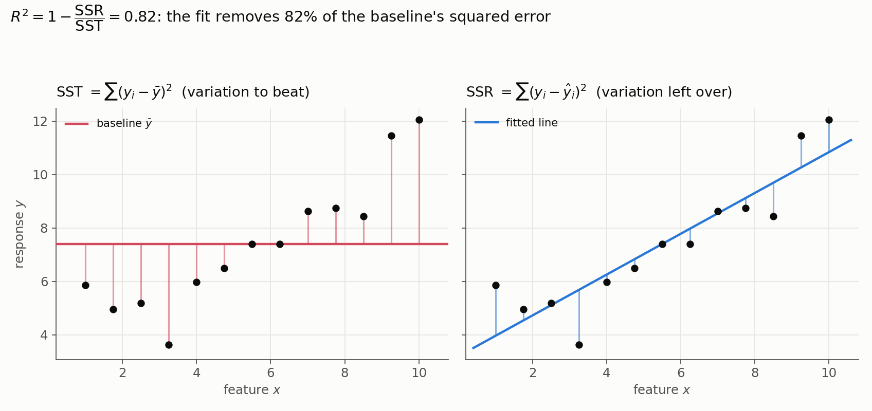
The left panel is the error to beat; the right panel is what the model leaves behind. Here the fit shrinks the residual segments enough to remove 82% of the baseline’s squared error, so $R^2 = 0.82$.

Important Caveats and Limitations

While R-squared is very useful, we should be aware of its limitations:

1. R-squared Always Increases with More Predictors: If we add more features to our model (even irrelevant ones), the R-squared value will never decrease. It can be artificially inflated, making us think we have a better model when we are just adding complexity.

2. Adjusted R-squared: To counter the first limitation, we often use Adjusted R-squared. This modified version of R-squared penalizes the addition of predictors that do not improve the model more than would be expected by chance. It provides a more honest assessment of the model’s explanatory power.

3. A High R-squared Doesn’t Mean the Model is Good: A high R-squared could mean the model is overfit, especially if the number of predictors is high relative to the number of data points.

4. A Low R-squared Doesn’t Mean the Model is Bad: In some fields, such as social sciences or psychology, human behavior is very complex, and a model with an R-squared of 0.30 (30%) might be considered very significant and useful.

5. R-squared Can Go Negative Outside the Textbook Setting: The 0-to-1 guarantee holds only for an in-sample OLS fit with an intercept. Evaluated on held-out test data, or for a model fit without an intercept, or under constraints, $R^2$ can be negative - meaning the model predicts worse than a constant equal to the evaluation set’s mean. A negative test-set $R^2$ is a loud diagnostic, not a computation error.

In summary, R-squared is a valuable measure of how well our model’s features explain the variation in the target variable, but it should always be interpreted in the context of the specific problem and alongside other metrics.

---

2. Outliers: Impact, Detection, and Mitigation

This is a critical topic in building reliable machine learning models. The short answer is that standard linear regression is highly susceptible to outlier values.

Let’s break down why that is and the robust methods we can use to mitigate this issue.

Why is Linear Regression So Susceptible to Outliers?

The reason lies at the very core of how linear regression is trained: its cost function.

Standard linear regression aims to find the line that minimizes the Mean Squared Error (MSE). The formula for MSE is:

\[MSE = \frac{1}{n} \sum_{i=1}^{n} (y_i - \hat{y}_i)^2\]

The key is the squaring of the error term $(y_i - \hat{y}_i)$.

Imagine a single data point that is a significant outlier. It will be very far from the regression line, resulting in a large error. When we square this large error, it becomes disproportionately huge.

Example:

• A point with an error of 3 contributes $3^2 = 9$ to the total error.
• An outlier with an error of 30 contributes $30^2 = 900$ to the total error.

To minimize this massive squared error from the outlier, the optimizer will significantly shift the entire regression line towards that single outlier. This skews the model, making it a poor fit for the majority of the “inlier” data points.

An outlier with an extreme x-value, known as a high-leverage point, can be even more influential, acting like a pivot and dramatically changing the slope of the line.

How Can We Mitigate the Effect of Outliers?

There is a standard workflow for dealing with outliers: first detect them, then decide on a strategy to handle them.

1. Detecting Outliers

Before we can fix them, we have to find them. Common methods include:

• Visual Inspection: The simplest and often most effective method. Use scatter plots to visualize the relationship between variables and box plots to see the distribution of a single variable. Outliers will often be clearly visible.
• Statistical Methods:
  • Z-score: Measures how many standard deviations a data point is from the mean. A Z-score greater than 3 or less than -3 is often considered an outlier.
  • Interquartile Range (IQR): Data points that fall below Q1 - 1.5 * IQR or above Q3 + 1.5 * IQR are flagged as outliers. This is the method used by box plots.
• Cook’s Distance: This is a more advanced metric that specifically measures how much the regression model’s predictions would change if a particular data point were removed. A high Cook’s distance indicates a highly influential point.

2. Handling Outliers

Once an outlier is detected, we have several options:

a. Removal or Correction

• What it is: Simply delete the row containing the outlier.
• When to use it: This should be done with extreme caution. It is only appropriate if we can confirm that the outlier is due to a data entry error, measurement error, or is otherwise not representative of the population we are trying to model.
• Caveat: Never remove an outlier just because it’s an outlier. It might be a legitimate, though rare, data point that contains valuable information.

b. Data Transformation

• What it is: Apply a mathematical function to one or more variables. Taking the logarithm of a variable with a skewed distribution can pull in high values, reducing the impact of outliers. Other transformations include the square root or Box-Cox transformation.
• When to use it: When we have a skewed variable distribution and a non-linear relationship that can be linearized with a transformation.

c. Use Robust Regression Algorithms

This is often the most principled approach. Instead of changing the data, we change the model to one that is inherently less sensitive to outliers.

Here are some popular robust regression algorithms available in libraries like scikit-learn:

• Huber Regression:
  • How it works: This is a hybrid approach. For data points with small errors (inliers), it uses the Mean Squared Error (L2 loss). But for data points with large errors (outliers), it switches to using a less sensitive linear error, similar to Mean Absolute Error (L1 loss). This prevents the large errors from being squared and dominating the loss function.
  • Result: The influence of outliers is down-weighted, so they don’t pull the regression line as much.
• RANSAC (RANdom SAmple Consensus):
  • How it works: RANSAC is an iterative algorithm that tries to separate the data into inliers and outliers. It works by:
    1. Selecting a random subset of the data.
    2. Fitting a model to this subset (assuming they are inliers).
    3. Testing all other data points against this model and classifying them as inliers (if they are close to the line) or outliers (if they are far away).
    4. Repeating this process many times and selecting the model that was fit to the largest set of inliers.
  • Result: The final model is based only on the identified inliers, completely ignoring the outliers.
• Theil-Sen Regression:
  • How it works: This method calculates the slope between all possible pairs of points in the dataset and then takes the median of all these slopes. Since the median is robust to extreme values, the resulting slope is highly resistant to outliers.
  • Result: A very robust estimate of the model’s slope.

In summary, while standard linear regression is fragile, there is a rich set of tools and alternative algorithms available to create models that are much more robust to the presence of outliers.

---

3. Interpreting Linear Regression Coefficients

Interpreting coefficients is the bridge between a mathematical model and real-world actionable insights. However, this interpretation is fragile. It completely relies on specific conditions being met.

Here is the breakdown of how to read them and the strict rules required to trust them.

1. How to Interpret the Coefficients ($\beta$)

The interpretation depends on whether the feature (independent variable) is continuous or categorical.

Let’s use a standard housing price model equation:

\[\text{Price} = \beta_0 + \beta_1(\text{SqFt}) + \beta_2(\text{HasGarage}) + \epsilon\]

A. Continuous Variables (e.g., SqFt)

If $\beta_1 = 50$:

• The Interpretation: “For every 1 unit increase in Square Footage, the Price increases by \$50, holding all other variables constant.”
• Key Phrase: The phrase “holding all other variables constant” (ceteris paribus) is mandatory. It means this is the isolated effect of size, assuming the house doesn’t also gain a garage or change location.

B. Categorical/Binary Variables (e.g., HasGarage: 0 or 1)

If $\beta_2 = 15,000$:

• The Interpretation: “A house with a garage (value 1) costs \$15,000 more than a house without a garage (value 0), holding all other variables constant.”
• Note: This is always a comparison against the “baseline” (where the value is 0).

C. The Intercept ($\beta_0$)

If $\beta_0 = 30,000$:

• The Interpretation: “The predicted Price when all independent variables are zero.”
• Reality Check: Often, the intercept has no physical meaning (e.g., a house with 0 SqFt cannot exist). It is primarily there to anchor the regression line.

---

4. Does a Larger Coefficient Mean a More Important Feature?

The short answer is NO.

We cannot determine feature importance by simply comparing the raw values of the coefficients ($\beta_1$ vs $\beta_2$).

Here is the detailed explanation of why this is a trap and how to correctly compare them.

1. The Trap: The Scale of the Features

The size of a coefficient depends entirely on the units (or scale) of the corresponding feature variable.

The Example: Imagine we are predicting the Price of a House.

• $x_1$: Size of the house in Square Feet.
• $x_2$: Distance to the nearest school in Kilometers.

Let’s look at two scenarios representing the exact same physical reality:

Scenario A:

• $x_1$ (Size): Measured in Square Feet.
  • Coefficient $\beta_1 = 100$ (Price increases \$100 per sq ft).
• $x_2$ (Distance): Measured in Meters.
  • Coefficient $\beta_2 = -5$ (Price drops \$5 per meter away).

Comparison: $\beta_1 (100) > \beta_2 (-5)$. Conclusion: We might think “Size is more important.”

Scenario B: Now, let’s just change the unit of measurement for distance.

• $x_1$ (Size): Measured in Square Feet.
  • Coefficient $\beta_1 = 100$.
• $x_2$ (Distance): Measured in Kilometers (1 km = 1000 meters).
  • Since 1 km is 1000x larger than 1 meter, the coefficient must be 1000x larger to have the same effect.
  • Coefficient $\beta_2 = -5000$ (Price drops \$5000 per km away).

Comparison: $|\beta_2| (5000) \gg \beta_1 (100)$. Conclusion: Now it looks like “Distance is vastly more important.”

The Reality: The underlying importance of the feature didn’t change, only the units did. Therefore, raw coefficients are meaningless for comparison.

2. The Solution: Standardized Coefficients

To compare $\beta_1$ and $\beta_2$ fairly, we must standardize our features (scale them) before training the model.

Standardization puts all features on the same playing field (usually Mean = 0, Standard Deviation = 1).

\[z = \frac{x - \mu}{\sigma}\]

If we train a regression model on these standardized features:

1. The units (feet, meters, years) disappear.
2. The coefficients represents the change in Y given a 1 standard deviation increase in X.
3. Result: We CAN compare these coefficients - with the right claim attached. If $\lvert \beta_{std, 1} \rvert > \lvert \beta_{std, 2} \rvert$, then $x_1$ has the larger within-model association with the target. Whether that makes it more “important” depends on which question is being asked - see the summary below.

3. The Other Trap: Statistical Significance

Even if we standardize our data, there is one more catch.

Imagine:

• $\beta_1 = 50$
• $\beta_2 = 5$

Can we say $x_1$ is 10x more important? Not necessarily. We must check the Standard Error and P-values.

• $x_1$ might have a huge standard error. Its 95% confidence interval might be $[-100, 200]$. This means we aren’t even sure if the effect is positive or negative! It is statistically insignificant.
• $x_2$ might have a tiny standard error. Its confidence interval might be $[4.9, 5.1]$. It is statistically significant.

In this case, despite $\beta_1$ being larger, $x_2$ is the “more important” (or at least more reliable) predictor because $x_1$ is just noise.

Summary: Ask What Kind of Importance First

Standardization plus significance is necessary hygiene, but it is still not a complete recipe - because statistical significance measures evidence against a null hypothesis, not importance. Correlated features, interactions, nonlinearity, and the precision of each estimate all blur any single ranking. The honest workflow is question-first:

• Within-model association: compare standardized coefficients - a limited comparison that scaling and significance make defensible, not definitive.
• Uncertainty: report confidence intervals, not just point estimates. Two coefficients with heavily overlapping intervals have no meaningful ranking.
• Incremental explanatory value: compare partial $R^2$, or nested models fit with and without the feature.
• Predictive contribution: use permutation importance, or the drop in held-out performance when the feature is removed.
• Causal effect: if “important” means “changing it changes the outcome,” no coefficient comparison substitutes for a causal design - that is a different question with different tools.

“Which feature matters most?” has several defensible answers; the trap is answering one version of the question with the machinery of another.

---

5. Generalized Linear Models vs. Vanilla Linear Regression

A Generalized Linear Model (GLM) is a more flexible and powerful framework that encompasses “vanilla” linear regression as just one of its many variations. While a standard linear regression assumes the outcome variable is continuous and normally distributed, a GLM can handle wildly different types of outcomes (like binary clicks or daily counts) by using a link function and assuming a different underlying probability distribution.

In essence, linear regression is just a specific, highly constrained type of GLM.

Vanilla Linear Regression

A standard linear regression model works under a strict set of assumptions:

1. Relationship: It models a direct linear relationship between the features ($X$) and the expected outcome ($Y$).

   \[Y = \beta_0 + \beta_1X_1 + \dots + \beta_pX_p + \epsilon\]
2. Distribution: It assumes the errors ($\epsilon$) are normally distributed, which makes the conditional response normal: $Y \mid X \sim \mathcal{N}(X\beta, \sigma^2)$. (As Part 1 showed, this is a statement about $Y$ given the features - the marginal distribution of $Y$ need not be normal.)
3. Outcome Type: It is only suitable for predicting continuous, unbounded target variables (e.g., price, temperature, height).

Classic Example: Predicting a house price. The price is a continuous number, and we assume it goes up or down linearly with features like square footage.

The Generalized Linear Model (GLM) Framework

A GLM breaks free from the normal distribution by standardizing models into Three Pillars:

1. The Random Component (Probability Distribution): Instead of forcing a Normal distribution, we can choose a distribution from the exponential family that actually matches the outcome’s shape.
   • Binomial: For binary outcomes (e.g., Converted vs. Not Converted).
   • Poisson: For count data (e.g., number of sessions, number of defects).
   • Gamma: For heavily skewed continuous data (e.g., customer lifetime value).
   • Gaussian (Normal): For standard continuous data - with the identity link $g(\mu) = \mu$, this reproduces vanilla linear regression exactly.

2. The Systematic Component (Linear Predictor): Just like vanilla regression, the GLM calculates a linear combination of the input features. We usually denote this linear predictor as $\eta$ (eta).

   \[\eta = \beta_0 + \beta_1X_1 + \dots + \beta_pX_p\]

3. The Link Function ($g$): This is the crucial innovation. We cannot always draw a straight line through complex data without predicting impossible values (like negative counts or probabilities > 100%). The link function $g(\mu)$ connects the conditional mean of the outcome ($\mu = E[Y \mid X]$) to the linear predictor ($\eta$).

   \[g(\mu) = \eta\]

   Geometrically, the link function translates the bounded reality of our data into the unbounded $[-\infty, \infty]$ space so the linear math can do its job without breaking.

The Cheat Sheet Comparison

Feature	Vanilla Linear Regression	Generalized Linear Model (GLM)
Target Variable Type	Continuous & Unbounded	Continuous, Binary, Counts, Skewed
Random Component	Normal (Gaussian)	Any from the exponential family (Binomial, Poisson, etc.)
Systematic Component	Models $Y$ directly	Models a transformation of $Y$’s mean via a link function

Example 1: Modeling Customer Complaints (Count Data)

Let’s say a company wants to predict the number of customer complaints received per day based on the number of sales made that day.

Why Vanilla Linear Regression Fails

If we use a standard linear regression model: $\text{complaints} = \beta_0 + \beta_1 \cdot \text{sales}$, We run into two major problems:

1. Nonsensical Predictions: The model shoots a straight line into infinity. It could easily predict a negative number of complaints (e.g., $-0.7$) on a day with very few sales, which is impossible.
2. Incorrect Distribution: Complaints are count data. The distribution is bounded at zero and heavily right-skewed (most days have 0, 1, or 2 complaints - very few have 10+). A normal bell curve is a terrible fit.

How a GLM (Poisson Regression) Succeeds

We can use a GLM specifically designed for count data.

1. Random Component: We select the Poisson distribution, which perfectly models event counts.
2. Systematic Component: The linear engine remains $\eta = \beta_0 + \beta_1 \cdot \text{sales}$.

3. Link Function: We use the Log link function. The model predicts the logarithm of the expected count ($\mu$).

   \[\ln(\mu) = \beta_0 + \beta_1 \cdot \text{sales}\]

Why this works: To get the actual predicted count of complaints, we take the exponential of the model’s output: $\mu = e^{(\beta_0 + \beta_1 \cdot \text{sales})}$. Because an exponential curve never dips below zero, our model will always predict a positive count, fixing the nonsensical prediction problem mathematically!

Two precision notes on Poisson models: it is the conditional mean $\mu$ that stays positive - observed counts can still be zero, and zero is a perfectly ordinary Poisson outcome. And the Poisson family’s built-in assumption that the variance equals the mean is frequently violated by real data (overdispersion); when that happens, Negative Binomial regression is the standard next step.

Example 2: Modeling A/B Test Conversions (Binary Data)

This same framework is the secret engine behind A/B testing. If we want to predict whether a user will Convert (1) or Not Convert (0) based on which Variant they saw, a vanilla linear line would predict impossible conversion rates like 1.2 (120%) or $-0.15$ (-15%).

By switching the GLM components:

1. Random Component: Binomial Distribution
2. Link Function: Logit function $g(\mu) = \ln(\frac{\mu}{1-\mu})$

We create Logistic Regression. The logit link function geometrically bends the straight line into an S-curve, ensuring the predicted conversion rates stay strictly bounded between 0 and 1.

The “Signal vs. Noise” Principle - Why We Model Expected Values

If we look closely at the math for Generalized Linear Models, we notice something subtle but crucial: we never write an equation that says $g(Y) = \dots$. Instead, we write $g(E[Y]) = \dots$ (or $g(\mu)$).

Why do we go through the trouble of modeling the Expected Value of $Y$ ($E[Y]$) instead of just modeling $Y$ directly? And why don’t we apply that same expectation to our features ($X$)?

The answer comes down to separating the “signal” from the “noise,” and understanding exactly what a predictive model is actually asking.

1. The “One Input, Many Outputs” Problem

Imagine we have two users in an A/B test who are perfectly identical on paper. They share the exact same device, location, historical purchase behavior, and they both saw the Treatment variant.

• User A clicks the button ($Y = 1$).
• User B does not click the button ($Y = 0$).

If we tried to model $Y$ directly using a strict mathematical function based on user features, the model would break. A mathematical function can only output one answer for a given set of inputs, it cannot output both 1 and 0 simultaneously.

Because human behavior contains inherent randomness, we cannot perfectly predict the exact, discrete outcome ($Y$) of a single, specific event. However, we can accurately predict the average or probable outcome across many identical events. That is the expected value. In this case, the model might output an expected value of $0.50$, meaning a perfectly identical user has a 50% chance of clicking.

2. Separating the Signal from the Noise

In statistics, every single data point we collect ($Y$) is made of two parts:

1. The Signal: The true underlying pattern driven by our features (e.g., the actual impact of our new A/B test variant).
2. The Noise: The random, unpredictable chaos of the real world (e.g., the user got distracted by a phone call and closed the app).

Vanilla Linear Regression explicitly shows this by adding an error term ($\epsilon$) at the end of the equation to represent the noise:

\[Y = \beta_0 + \beta_1X + \epsilon\]

Here is the mathematical magic: what happens if we want to find the average/expectation of both sides of that vanilla equation?

• The expectation of $Y$ becomes $E[Y]$.
• The expectation of the linear math $(\beta_0​+\beta_1 ​X)$ stays exactly the same, because it is fixed.
• The expectation of the random error term $(E[\epsilon])$ is exactly zero, because random noise cancels itself out on average.

So, taking the expectation of the standard linear regression equation simplifies perfectly to:

\[E[Y] = \beta_0​+\beta_1 ​X\]

GLMs simply take this cleaner, noise-free $E[Y]$ equation and wrap it in a link function! By modeling the expectation, GLMs elegantly separate the messy reality of individual data points from the underlying mathematical truth we are trying to discover.

3. The Secret of Conditional Expectation: Why not $E[X]$?

This brings us to a common point of confusion. If we take the expectation of the equation, why does it become $E[Y] = \beta_0 + \beta_1X$? Why don’t we take the expectation of $X$ as well, writing it as $E[Y] = \beta_0 + \beta_1 E[X]$?

The reason lies in a mathematical shorthand. The full, mathematically correct notation isn’t actually $E[Y]$. It is $E[Y \vert X]$.

That vertical bar | means “given”.

When we build a regression model, we aren’t trying to find the average outcome of the entire universe. We are asking: “What is the expected outcome $Y$, given that we already know the exact value of $X$?”

• The Rule of Constants: Because we are treating $X$ as a known, fixed piece of information for a specific prediction, $X$ is no longer a random variable that fluctuates. It becomes a constant. And the expected value of a constant is just the constant itself (e.g., the expected value of 5 is just 5).
• Because $X$ is known, $E[X] = X$.

What would happen if we actually used $E[X]$?

$E[X]$ represents the overarching global average of a feature across the entire population. In an A/B test split 50/50, the average variant assignment ($X$) across everyone is $0.5$.

If we used $E[X]$ in the formula, our model would look like this for every single user:

\[E[Y] = \beta_0 + \beta_1(0.5)\]

By taking the expectation of $X$, we destroy the individual user’s data! We would predict the exact same, watered-down “global average” conversion rate for every single person, completely ignoring whether they actually saw the Control or the Treatment.

The Takeaway: GLMs elegantly separate the messy reality of individual data points from the underlying mathematical truth. We model $E[Y|X]$ because we want to isolate the pure signal of the outcome, conditional on the specific, known facts we have about our users.

---

Closing Perspective

Linear regression is more than a formula for fitting a straight line. It is a connected framework: assumptions justify the estimator, diagnostics expose its weaknesses, regularization stabilizes it, evaluation measures its usefulness, and GLMs extend its core idea to outcomes that a Gaussian response cannot describe.

Taken together, the three parts move from how the solution is derived, through how it fails and can be repaired, to how it should be evaluated, interpreted, and extended.