Logistic Regression, Part 2: Coefficients, Decision Boundaries, and Limitations

Logistic Regression series: Part 1: From Log-Odds to Gradient Descent · Part 2: Coefficients, Decision Boundaries, and Limitations · Part 3: Softmax, Neural Networks, and Imbalanced Data

Part 1 derived the binary model and showed how cross-entropy turns observed labels into fitted coefficients. This part asks what the fitted model means.

We will move from log-odds to odds ratios and probability changes, examine how scaling affects interpretation and regularization, derive the decision boundary for any threshold, and use XOR to expose the limitation of a linear score.

---

1. Interpreting Coefficients and Odds Ratios

Interpreting the coefficients in logistic regression isn’t as straightforward as in linear regression (where they represent a simple slope), but it’s incredibly insightful once we understand the concept of odds.

The key is to realize that logistic regression models the log-odds of an event happening. Therefore, the coefficients must be interpreted in relation to this scale.

The Foundation: From Log-Odds to Odds Ratios

The logistic regression equation is:

\[\ln\left(\frac{P}{1-P}\right) = \beta_0 + \beta_1 X_1 + \beta_2 X_2 + \dots + \beta_k X_k\]

Let’s break this down:

• P: The probability of the event of interest occurring (e.g., the team winning).
• P / (1-P): This is the odds of the event. It’s the ratio of the probability of the event happening to the probability of it not happening.
• ln(P / (1-P)): This is the log-odds or logit. The logistic regression model predicts this value.
• β₁…βk: These are the coefficients for each predictor variable. They represent the change in the log-odds for a one-unit change in the predictor.

Because “log-odds” are not intuitive for most people, we exponentiate the coefficient to get an Odds Ratio (OR).

\[OR = e^\beta\]

The Odds Ratio is the most common and intuitive way to interpret the coefficients. It tells us how the odds of the outcome event change for a one-unit increase in the predictor variable, holding all other variables constant.

Derivation of the Odds Ratio (OR)

Remember the fundamental equation:

\[\log(\text{odds}) = \beta_0 + \beta_1 X_1 + \beta_2 X_2 + ...\]

Let’s focus on interpreting the coefficient $\beta_1$ for the predictor $X_1$.

Scenario 1: The odds at some value of $X_1$

Let’s calculate the predicted odds for a specific observation where $X_1$ has some value, and all other predictors ($X_2$, $X_3$, etc.) are held at constant values.

\[\text{odds}_1 = e^{(\beta_0 + \beta_1 X_1 + \beta_2 X_2 + ...)}\]

Scenario 2: The odds when $X_1$ increases by one unit

Now, let’s see what happens to the odds when we increase only $X_1$ by one unit (from $X_1$ to $X_1 + 1$), keeping everything else the same.

\[\text{odds}_2 = e^{(\beta_0 + \beta_1 (X_1 + 1) + \beta_2 X_2 + ...)}\]

Calculating the Odds Ratio (OR)

The odds ratio is the ratio of the odds in Scenario 2 to the odds in Scenario 1. It tells us how much the odds were multiplied by when we increased $X_1$ by one.

\[\text{OR} = \text{odds}_2 / \text{odds}_1\]

Now let’s substitute the equations. Look at what happens inside that exponent. Almost every term cancels out!

• $\beta_0 - \beta_0 = 0$
• $\beta_1 X_1 - \beta_1 X_1 = 0$
• $\beta_2 X_2 - \beta_2 X_2 = 0$
• …and so on for all other variables.

The only term that doesn’t cancel out is the single $\beta_1$ from the numerator.

So, the entire expression simplifies to:

\[\text{OR} = e^{\beta_1}\]

Conclusion

This is why $e^{\beta}$ is the odds ratio. It isolates the effect of a single predictor by showing the multiplicative change in the odds. The other terms all cancel out when we calculate the ratio of the odds, leaving us with just the exponentiated coefficient for the variable we’re interested in.

How to Interpret the Odds Ratio (OR)

Let’s look at the different scenarios for an Odds Ratio:

• If OR > 1: For a one-unit increase in the predictor, the odds of the outcome occurring increase by a factor of the OR. It’s associated with a higher likelihood of the event.
• If OR < 1: For a one-unit increase in the predictor, the odds of the outcome occurring decrease by a factor of the OR. It’s associated with a lower likelihood of the event.
• If OR = 1: The predictor has no effect on the odds of the outcome.

Interpreting Different Types of Variables

The interpretation varies slightly depending on whether the predictor is continuous or categorical.

1. For a Continuous Variable

Let’s use the example: predicting a win based on no_of_hours_practiced.

Assume our logistic regression model gives us a coefficient $\beta_1 = 0.05$ for the no_of_hours_practiced variable.

1. Direct Coefficient Interpretation (Log-Odds):
   • For each additional hour of practice, the log-odds of the team winning increases by 0.05, holding all other factors constant. (This is correct, but not very intuitive).
2. Odds Ratio Interpretation (More Intuitive):
   • First, calculate the Odds Ratio: $OR = e^{0.05} \approx 1.051$
   • Interpretation: For each additional hour of practice, the odds of the team winning increase by a factor of 1.051, or about 5.1%.

2. For a Categorical Variable

Now let’s add a categorical variable to our model, for example, match_location with two categories: “Home” and “Away”.

To include this in the model, we use dummy coding. We create a variable, let’s call it is_home_match, where:

• is_home_match = 1 if the match is at home.
• is_home_match = 0 if the match is away (this is our “reference” or “baseline” category).

Suppose the model gives a coefficient $\beta_2 = 0.693$ for is_home_match.

1. Direct Coefficient Interpretation (Log-Odds):
   • The log-odds of winning for a home match are 0.693 higher than for an away match, holding practice hours constant.
2. Odds Ratio Interpretation (More Intuitive):
   • Calculate the Odds Ratio: $OR = e^{0.693} \approx 2.0$
   • Interpretation: The odds of winning when playing at home are twice as high as the odds of winning when playing away, assuming the same number of practice hours.

A Practical Example Summary

Imagine our final model is:

\[\ln(\text{odds\_of\_winning}) = -3.0 + 0.05 \times (\text{hours\_practiced}) + 0.693 \times (\text{is\_home\_match})\]

And the corresponding Odds Ratios are:

• For hours_practiced: $e^{0.05} \approx 1.051$
• For is_home_match: $e^{0.693} \approx 2.0$

We would report this as:

“Controlling for match location, each additional hour of practice increases the odds of winning by 5.1%. Furthermore, controlling for practice hours, the odds of winning a home match are double the odds of winning an away match.”

Odds Changes Are Not Probability Changes

An odds ratio is multiplicative on the odds, not additive on the probability. If $\beta_1=0.05$, each extra hour multiplies the odds by $e^{0.05}\approx1.051$; it does not add 5.1 percentage points to the win probability.

The probability effect depends on the starting probability. For a continuous feature, the instantaneous marginal effect is:

\[\frac{\partial p}{\partial x_j}=\beta_jp(1-p).\]

The same coefficient therefore produces its largest probability change near $p=0.5$ and a smaller change near 0 or 1. When communicating results, report predicted probabilities at meaningful feature values alongside odds ratios.

These interpretations also assume that the model is correctly specified and that other predictors are held constant. With interaction terms, the effect of one feature depends on the value of the feature it interacts with.

---

2. What Feature Scaling Changes

The short answer is: No, we do not need to scale features to interpret coefficients as odds ratios. Scaling mainly changes coefficient units, numerical conditioning, and how regularization treats different features.

Here’s the detailed breakdown of the trade-off:

Case 1: We DO NOT Scale the Features

This is often preferred when our main goal is straightforward, intuitive interpretation.

• How it works: The interpretation of $e^\beta$ remains the same: “A one-unit increase in the predictor X is associated with a multiplicative change of $e^\beta$ in the odds of the outcome.”
• The “Unit” is Natural: The key is that the “one-unit” is in the original, natural scale of the data.
  • If the predictor is age in years, a one-unit change is one year.
  • If the predictor is price in dollars, a one-unit change is one dollar.
  • If the predictor is distance in kilometers, a one-unit change is one kilometer.

• Advantage: This is the easiest interpretation to explain to a non-technical audience. “For every additional year of age, the odds of purchasing the product increase by 5%” is much clearer than talking about standard deviations.

• Disadvantage:
  1. Model Convergence: If the features are on wildly different scales (e.g., age from 20-80 and income from 20,000-200,000), the gradient descent algorithm used to train the model can struggle and may take longer to converge.
  2. Cannot Compare Coefficients: We cannot compare the magnitude of the coefficients to infer feature importance. A coefficient of 0.05 for income is not necessarily less important than a coefficient of 1.2 for number_of_children, because a “one-unit” change means something completely different for each.

Case 2: We DO Scale the Features

Standardization gives each numeric feature mean 0 and standard deviation 1. It is particularly useful when optimization is sensitive to feature scale or when the model uses a coefficient penalty.

• How it works: Again, the interpretation of $e^\beta$ is for a “one-unit” change in the predictor.

• The “Unit” is Standard Deviations: But now, because the feature has been standardized, a “one-unit” change means a one standard deviation increase from the mean.

• Advantages:
  1. Better numerical conditioning: Some iterative solvers converge faster and more reliably when features have comparable scales.
  2. Comparable regularization: Ridge, Lasso, and Elastic Net penalize coefficient magnitude, so unscaled units can make the penalty act unevenly.
  3. A common coefficient unit: Each coefficient describes a one-standard-deviation increase, which permits a limited comparison of changes in log-odds.
• Disadvantage: The interpretation is less direct. We have to phrase it as: “For every one standard deviation increase in age, the odds of the outcome increase by a factor of $e^\beta$.” We then have to follow up by explaining what one standard deviation of age is in our data (e.g., “which is equivalent to 12.5 years”).

Summary and Recommendation

Goal	To Scale or Not?	Why?
Natural-unit interpretation	Usually leave units unchanged	A one-unit change remains one year, dollar, or kilometer.
Numerically sensitive solver	Scale	Comparable feature ranges can improve convergence.
L1/L2 regularization	Scale numeric features	The penalty then treats coefficients on a comparable basis.
Coefficient comparison	Scale, but interpret cautiously	Standardization aligns units; it does not establish predictive or causal importance.

For an unregularized model solved to convergence, rescaling a feature does not inherently improve statistical fit: the coefficient changes units while fitted probabilities can remain the same. There is also no need to train a second model merely to recover natural-unit interpretations. If $x’=(x-\mu)/s$, transform the coefficient back algebraically:

\[\beta_{\text{original}}=\frac{\beta_{\text{scaled}}}{s}.\]

The intercept changes as well. With regularization, however, scaling changes the optimization problem, so this equivalence requires more care.

---

3. In What Sense Is Logistic Regression Linear?

Yes, logistic regression is a linear model, but the phrase “linear model” refers to something very specific. Once we understand what is linear and where, the confusion disappears.

Let’s break it down cleanly.

Short Answer

Yes, logistic regression is a linear model because:

It is linear in the parameters (the weights), not in the output.

This is the key idea.

Long Answer: What “Linear” Actually Means

In ML/statistics, a linear model is one where the prediction is a linear combination of the input features:

\[z = \beta_0 + \beta_1 x_1 + \beta_2 x_2 + \cdots + \beta_d x_d\]

This part is 100% linear.

Logistic regression takes that linear score (z) and passes it through a nonlinear link function (the sigmoid):

\[\hat{y} = \sigma(z) = \frac{1}{1 + e^{-z}}\]

The sigmoid squashes the result into a probability between 0 and 1, that’s the only nonlinearity.

So:

• Linear in the weights → yes
• Linear in the supplied feature representation before the sigmoid → yes
• Final output linear? → no, because of sigmoid

And that’s okay, the model is still classified as a generalized linear model (GLM).

What Is NOT Linear About It

• The decision boundary is linear in the features supplied to the model.

  • Example: $\beta_0 + \beta_1 x_1 + \beta_2 x_2 = 0$

• But the probabilities are nonlinear due to the sigmoid.

That’s why logistic regression is both:

• linear (in parameters / decision boundary)
• nonlinear (in output probabilities)

If we supply transformed features such as $x_1^2$, splines, or $x_1x_2$, the model remains linear in its coefficients but can create a nonlinear boundary when viewed in the original raw-feature space.

---

4. Deriving the Decision Boundary

Logistic regression is a linear classifier, which means it finds a linear decision boundary to separate two classes.

How it Works

The core of logistic regression is a linear equation, just like in linear regression:

\[\text{z} = \beta_0 + \beta_1 \text{x}_1 + \beta_2 \text{x}_2 + ...\]

This equation calculates a score based on the input features ($\text{x}_1$, $\text{x}_2$, etc.). The model then makes its decision based on the sign of this score.

The decision boundary is the line (or plane/hyperplane in more dimensions) where the model is exactly uncertain about which class to predict. For logistic regression, this happens when the probability is 50%, which corresponds to the score z being exactly 0.

Therefore, the equation for the decision boundary is:

\[\beta_0 + \beta_1 \text{x}_1 + \beta_2 \text{x}_2 + ... = 0\]

This is the boundary for the usual probability threshold $t=0.5$, since $\operatorname{logit}(0.5)=0$. For a different decision threshold $t$, the boundary shifts to:

\[\beta_0+\beta^Tx=\log\left(\frac{t}{1-t}\right).\]

Changing the threshold moves the hyperplane without changing its orientation. This is important when false positives and false negatives have different costs.

Visualization

Imagine we have two features, $\text{x}_1$ and $\text{x}_2$. The logistic regression model will find the single best straight line that separates the data points of Class A from Class B.

Key Point: Even though the sigmoid probability is nonlinear, the boundary is linear in the supplied feature representation. With only the two raw XOR inputs, that representation is not linearly separable.

---

5. XOR and the Limit of Linear Separability

The answer is no when the model receives only the two raw XOR inputs. A linear boundary in that feature space cannot separate the classes.

Here’s a clear explanation of why.

1. What is the XOR Problem?

XOR stands for “exclusive OR”. It’s a simple logical operation that outputs true (or 1) only when the inputs are different.

Let’s look at the truth table and visualize it on a graph:

Input 1 (X₁)	Input 2 (X₂)	Output (Y)
0	0	0
0	1	1
1	0	1
1	1	0

When we plot these points, we get this pattern:

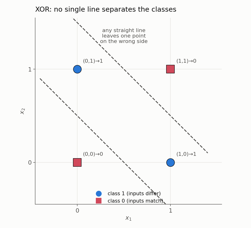
The two classes sit on opposite diagonals. Whichever straight line we try - the two dashed attempts above are typical - one point always lands on the wrong side. That is the visual signature of a non-linearly separable problem.

2. The Limitation of Logistic Regression: Linear Separability

The core of a logistic regression model is a linear equation:

\[\text{z} = \beta_0 + \beta_1 \text{x}_1 + \beta_2 \text{x}_2\]

The model’s decision boundary, the line where it is uncertain (probability = 0.5), occurs when z = 0. This means the boundary is defined by the equation β₀ + β₁X₁ + β₂X₂ = 0, which is the equation of a straight line.

A logistic regression model works by finding the best single straight line to separate the two classes (the 0s from the 1s).

3. Why It Fails for XOR

Now, look back at the XOR plot.

Can we draw one single straight line that separates the blue points (class 1) from the red points (class 0)?

We can’t.

• If we draw a line to separate (0,0) from the others, we group (1,1) with the wrong class.
• If we draw a diagonal line, we can separate two points, but we will always misclassify the other two.

The XOR problem is the classic example of a non-linearly separable problem. With only $x_1$ and $x_2$, logistic regression cannot correctly classify all four points. The limitation belongs to the feature representation, not to the sigmoid itself.

How Can the XOR Problem Be Solved?

This very limitation is what led to the development of more complex models. The XOR problem can be solved by:

1. Neural Networks: A simple neural network with just one hidden layer containing two neurons can solve it. The hidden layer learns to transform the data into a new representation where it is linearly separable.
2. Kernel SVMs: A Support Vector Machine (SVM) using a non-linear kernel (like the Radial Basis Function or Polynomial kernel) can project the data into a higher dimension where a separating hyperplane (the equivalent of a line) can be found.
3. Feature Engineering: We could manually create a new feature, X₃ = X₁ * X₂. If we add this feature to the logistic regression model, it can then find a linear boundary in this new 3D space to solve the problem.

---

A binary logistic model uses one linear score and one sigmoid output. Part 3 uses that same structure as a bridge to neural networks and multiclass softmax, then closes with evaluation and training choices for imbalanced datasets.