Naive Bayes: From Bayes' Rule to Text Classification

Naive Bayes remains a cornerstone baseline for classification, especially on sparse, high-dimensional text. Despite the “naive” label, it rests on a clean probabilistic model. In this article we derive that model once, work a complete numerical spam example in log space, tour the whole family of variants, and then get the parts that are easy to state loosely, MAP decisions, smoothing, and probability calibration, exactly right.

1. What Naive Bayes Models

We observe a feature vector $x = (x_1, x_2, \dots, x_d)$ and want to assign it a class label $C$. Bayes’ theorem relates the quantity we want to the quantities we can estimate:

\[P(C = c \mid x) = \frac{P(x \mid C = c)\, P(C = c)}{P(x)}.\]

Reading off the four terms: $P(C = c)$ is the prior (how common the class is), $P(x \mid C = c)$ is the likelihood (how compatible the features are with the class), $P(x)$ is the evidence, and $P(C = c \mid x)$ is the posterior (what we actually want). Because the evidence $P(x)$ is the same for every class, it cannot change which class scores highest, so we drop it:

\[P(C = c \mid x) \propto P(C = c)\, P(x_1, x_2, \dots, x_d \mid C = c).\]

The remaining likelihood is a full joint distribution over all $d$ features. Estimating it directly is not mathematically impossible, but it is statistically impractical: the number of distinct feature combinations grows exponentially in $d$, so we would need an enormous training set to see each combination often enough to estimate its probability. This is the curse of dimensionality.

The “Naive” Assumption

Naive Bayes sidesteps that problem with one bold assumption: the features are conditionally independent given the class. Formally, $x_i$ is assumed independent of $x_j$ once we know $C$. That collapses the joint likelihood into a product of one-dimensional factors:

\[P(x_1, x_2, \dots, x_d \mid C = c) = \prod_{j=1}^{d} P(x_j \mid C = c).\]

Each factor $P(x_j \mid C = c)$ is a simple one-feature distribution we can estimate reliably. The decision rule becomes:

\[\hat c = \arg\max_{c} \; P(C = c) \prod_{j=1}^{d} P(x_j \mid C = c).\]

Score in Log Space

Multiplying hundreds or thousands of probabilities together drives the product toward zero fast enough to underflow floating-point arithmetic. Every production implementation therefore works with the logarithm of the score:

\[\hat c = \arg\max_{c} \left[ \log P(C = c) + \sum_{j=1}^{d} \log P(x_j \mid C = c) \right].\]

Because the logarithm is monotonic, this picks the same class as the raw product, but sums of log-probabilities stay in a safe numeric range. When we need normalized posterior probabilities rather than just the winning label, we convert the joint log-scores back with the log-sum-exp trick. We use log-space scoring for the worked example below, and it is worth treating as the default rather than an implementation footnote.

One reassuring fact before we compute anything: Naive Bayes often classifies well even when the independence assumption is false. Only the ranking of class scores has to be correct for the prediction to be right, and that ranking can survive estimation errors that would ruin the individual probabilities.

2. A Worked Spam Classification

Let us make the machinery concrete with a tiny spam-versus-ham corpus. We use ham to mean a legitimate (non-spam) email throughout. Restrict attention to a three-word vocabulary, $\{\text{free}, \text{meeting}, \text{money}\}$, and take ten training emails:

• Spam (4): “free money money”, “free money”, “free free money”, “free money”
• Ham (6): “meeting meeting”, “free meeting”, “meeting meeting”, “meeting”, “free meeting”, “meeting”

From these documents we read off two kinds of statistics: token counts (how many times each word occurs, used by Multinomial Naive Bayes) and document presence (how many documents contain each word at least once, used by Bernoulli Naive Bayes).

Class	Docs	free (count / docs)	meeting (count / docs)	money (count / docs)	Total tokens
Spam	4	5 / 4	0 / 0	5 / 4	10
Ham	6	2 / 2	8 / 6	0 / 0	10

The empirical class priors are $P(S) = 4/10 = 0.4$ and $P(H) = 6/10 = 0.6$. Our task: classify the new email “free money”.

Multinomial Scoring

Multinomial Naive Bayes estimates each word probability from token counts with additive smoothing, adding $\alpha = 1$ to every count and $\alpha \lvert V \rvert = 3$ to each denominator so the probabilities still sum to one:

\[P(w \mid c) = \frac{\text{count}(w, c) + \alpha}{\text{(total tokens in } c) + \alpha \lvert V \rvert}.\]

Both denominators are $10 + 3 = 13$, giving:

Word	$P(w \mid S)$	$P(w \mid H)$
free	$6/13 \approx 0.462$	$3/13 \approx 0.231$
money	$6/13 \approx 0.462$	$1/13 \approx 0.077$

Note that “money” never appears in ham, so its ham probability rests entirely on smoothing. Scoring “free money” in log space:

\[\log P(S) + \log P(\text{free} \mid S) + \log P(\text{money} \mid S) = \log 0.4 + 2\log\tfrac{6}{13} \approx -2.46,\] \[\log P(H) + \log P(\text{free} \mid H) + \log P(\text{money} \mid H) = \log 0.6 + \log\tfrac{3}{13} + \log\tfrac{1}{13} \approx -4.54.\]

Spam wins. Exponentiating and normalizing the two joint scores gives $P(\text{spam} \mid \text{“free money”}) \approx 0.89$. Scikit-learn’s MultinomialNB returns the same 0.89 on this corpus.

Bernoulli Scoring

Bernoulli Naive Bayes treats each word as a binary present-or-absent feature and estimates a presence probability $\theta_{wc} = P(\text{word } w \text{ present} \mid c)$ from document counts, smoothing with $\alpha = 1$ over the two outcomes:

\[\theta_{wc} = \frac{\text{(docs in } c \text{ containing } w) + \alpha}{\text{(docs in } c) + 2\alpha}.\]

Word	$\theta_{wS}$	$\theta_{wH}$
free	$5/6 \approx 0.833$	$3/8 = 0.375$
meeting	$1/6 \approx 0.167$	$7/8 = 0.875$
money	$5/6 \approx 0.833$	$1/8 = 0.125$

The crucial difference from Multinomial is that Bernoulli scores absent words too. Our email “free money” contains free and money but not meeting, so the meeting factor enters as $(1 - \theta_{\text{meeting}, c})$:

\[P(S)\,\theta_{\text{free},S}\,\theta_{\text{money},S}\,(1 - \theta_{\text{meeting},S}) = 0.4 \cdot \tfrac{5}{6} \cdot \tfrac{5}{6} \cdot \tfrac{5}{6} \approx 0.231,\] \[P(H)\,\theta_{\text{free},H}\,\theta_{\text{money},H}\,(1 - \theta_{\text{meeting},H}) = 0.6 \cdot \tfrac{3}{8} \cdot \tfrac{1}{8} \cdot \tfrac{1}{8} \approx 0.0035.\]

Normalizing gives $P(\text{spam}) \approx 0.985$, and BernoulliNB agrees. Bernoulli is even more confident than Multinomial here, and the absence term is why: ham emails almost always contain “meeting” ($\theta = 0.875$), so an email without it is strong evidence against ham. Multinomial never sees that signal, because a word with count zero simply contributes nothing to its product.

Out-of-Vocabulary Words

The vocabulary is fixed when the model is trained. A word that appears at prediction time but never during training has no estimated probability, so it must be handled deliberately: dropped, mapped to a shared unknown-token feature, or filtered by the vectorizer. It must never be silently assigned an undefined probability.

3. The Naive Bayes Family

The variants differ only in the feature model, the choice of $P(x_j \mid c)$. Scikit-learn ships five in common use:

Variant	Feature model	Typical use	Key caveat
Bernoulli NB	Binary presence / absence	Short text, binary indicators	Absence of a feature contributes evidence
Multinomial NB	Non-negative counts	Document and token classification	Repeated counts influence the score
Complement NB	Statistics from the other classes	Imbalanced text	Designed for count-like text features
Categorical NB	One categorical distribution per feature	Encoded discrete categories	Categories must be encoded consistently
Gaussian NB	Gaussian density per feature and class	Continuous measurements	Sensitive to non-Gaussian shapes and correlated features

Bernoulli and Multinomial Likelihoods

The two discrete variants encode genuinely different generative stories. For binary features $x_j \in \{0, 1\}$ with $\theta_{jc} = P(x_j = 1 \mid c)$, the Bernoulli likelihood multiplies a presence or absence factor for every word in the vocabulary:

\[P(x \mid c) = \prod_{j=1}^{d} \theta_{jc}^{\,x_j} (1 - \theta_{jc})^{\,1 - x_j}.\]

The $(1 - \theta_{jc})$ factors are exactly the absence terms we saw drive the worked example. The Multinomial score instead weights each word’s log-probability by its count, so a word that appears three times contributes three times:

\[\log P(c) + \sum_{j=1}^{d} x_j \log \theta_{jc}, \qquad \theta_{jc} = P(\text{term } j \mid c).\]

Multinomial features must be non-negative. Integer counts match the generative model exactly; fractional representations such as TF-IDF weights break the strict generative story but often work well in practice.

Gaussian Naive Bayes for Continuous Features

When features are continuous, such as height or temperature, we cannot count occurrences of an exact value. Gaussian Naive Bayes instead models each feature within each class as a normal distribution and evaluates its probability density. Note the lowercase $p$: this is a density, not the probability of observing one exact value (which is zero for any continuous variable).

\[p(x_j \mid C = c) = \frac{1}{\sqrt{2\pi \sigma_{jc}^2}} \exp\left[ -\frac{(x_j - \mu_{jc})^2}{2\sigma_{jc}^2} \right].\]

The model estimates a separate mean $\mu_{jc}$ and variance $\sigma_{jc}^2$ for every feature-class pair, then multiplies the per-feature densities (or, in log space, sums their logs).

A common misconception is that a value belongs to whichever class mean it sits closest to. That ignores variance. Suppose we classify iris flowers by petal length, with setosa tightly clustered at $\mu = 1.5$ cm, $\sigma = 0.2$ and versicolor more spread out at $\mu = 4.3$ cm, $\sigma = 0.5$. A petal of 2.5 cm is closer to the setosa mean in raw centimetres (1.0 cm away versus 1.8 cm), yet it is a 5-standard-deviation event for setosa and only 3.6 for versicolor. The versicolor density at 2.5 cm is roughly 165 times higher, so Gaussian Naive Bayes correctly prefers versicolor. Closeness to a mean alone does not determine the likelihood; the spread does too.

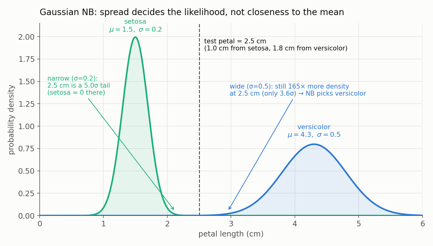
The narrow setosa curve has already collapsed to almost nothing by 2.5 cm, while the wide versicolor curve still carries real density there. Being close to a mean counts for little once the spread differs this much.

In practice, add a small variance floor (scikit-learn’s var_smoothing) so that a feature with near-zero variance in some class does not produce a division that blows up.

Complement and Categorical

Complement NB estimates each class’s parameters from the statistics of all the other classes, which makes it noticeably more stable than Multinomial on imbalanced text corpora. Categorical NB fits one categorical distribution per feature and is the natural choice when inputs are genuinely discrete categories (encoded consistently) rather than counts or measurements.

4. Smoothing and Parameter Estimation

The Zero-Frequency Problem

If a word never appears in a class during training, its unsmoothed likelihood is zero, and because we multiply likelihoods, that single zero annihilates all other evidence. Additive smoothing fixes this by adding a pseudo-count $\alpha$ to every count, as we did above. The naming depends on $\alpha$:

• $\alpha = 1$ is Laplace smoothing.
• $0 < \alpha < 1$ is Lidstone smoothing.

Crucially, $\alpha$ is a hyperparameter to tune, not a law of nature fixed at 1. Its best value depends on the corpus and belongs inside cross-validation.

Feature Smoothing Is Not Prior Smoothing

It is tempting to assume the same $\alpha$ automatically smooths the class priors as well, but that is an implementation choice, not a rule. Scikit-learn, for instance, controls feature smoothing through alpha while handling class priors separately through fit_prior and class_prior. Keep the two conceptually distinct.

Additive smoothing also has a clean Bayesian reading. Placing a symmetric Beta prior (for Bernoulli) or Dirichlet prior (for Multinomial) on the feature probabilities and taking the posterior-predictive probability reproduces the add-$\alpha$ formula, with $\alpha$ playing the role of the prior’s concentration. This is worth stating carefully: the add-$\alpha$ estimate is a posterior-predictive quantity, and equating it with a specific MAP estimate requires pinning down the exact prior parameterization.

5. MAP Classification Without Terminology Confusion

It is common to hear that “Naive Bayes is a MAP estimator,” but that phrase blurs two genuinely different operations.

Class prediction chooses the label with the largest posterior:

\[\hat c = \arg\max_{c} P(C = c \mid x).\]

This is a MAP decision over the class label, equivalently the Bayes-optimal decision under 0-1 loss. Parameter estimation is separate: it fits the class priors and feature parameters from the training data, and those estimates may come from maximum likelihood, smoothed frequencies, or a Bayesian posterior.

That distinction also clears up a second loose usage. A rule that ignores the prior and maximizes $P(x \mid c)$ alone is a maximum-likelihood classification rule. It coincides with the MAP rule only when the class priors are equal. Calling it “MLE” invites confusion, because MLE conventionally names a way of estimating parameters, not a way of choosing a label.

Finally, a word on the intuition that “the prior dominates with little data and the likelihood takes over as data grows.” That mixes two different meanings of the word prior. For a single prediction, the balance between $\log P(c)$ and $\sum_j \log P(x_j \mid c)$ depends on the feature vector in front of us, for text essentially the document length, not on the size of the training set. More training data makes the parameter estimates more stable; it does not mechanically shrink the class-prior term. It is in Bayesian parameter estimation that a prior over feature probabilities genuinely washes out as training counts grow. The two effects are worth keeping separate.

6. Strengths, Failure Modes, and Evaluation

Where it shines. Training and inference are fast and require only simple counting or moment estimates. With few parameters and no iterative optimization, Naive Bayes is an excellent baseline on sparse, high-dimensional problems like text, and it is hard to beat as a first model to ship.

Where it breaks. The independence assumption is the source of both its speed and its main weakness. When features are correlated, the model counts the same evidence repeatedly. Two near-duplicate words each contribute a full factor as if they were independent signals, which pushes the posterior toward 0 or 1. The result is a classifier whose labels are often still accurate but whose probabilities are overconfident and poorly calibrated. Gaussian Naive Bayes has an additional vulnerability: if a feature is far from Gaussian within a class, the density estimate is simply wrong. And if the class balance at deployment differs from training (prior shift), the fitted priors can steer decisions the wrong way until they are updated.

How to evaluate. For imbalanced labels, report F1 and PR-AUC rather than raw accuracy. When the probabilities themselves drive downstream decisions, measure them directly with log loss, the Brier score, and a calibration curve. If calibration is poor, fit Platt scaling or isotonic regression on held-out data to recalibrate the scores without disturbing the ranking.

7. A Practical Pipeline

The idiomatic scikit-learn setup pairs a vectorizer with a Naive Bayes estimator and tunes $\alpha$ by cross-validation:

from sklearn.pipeline import Pipeline
from sklearn.feature_extraction.text import CountVectorizer
from sklearn.naive_bayes import MultinomialNB, ComplementNB
from sklearn.model_selection import GridSearchCV

pipe = Pipeline([
    ("vec", CountVectorizer()),
    ("clf", MultinomialNB()),
])

# tune the smoothing strength inside cross-validation
grid = GridSearchCV(
    pipe, {"clf__alpha": [0.1, 0.5, 1.0]}, cv=5, scoring="f1_macro"
)
grid.fit(texts, labels)

# for imbalanced text, ComplementNB is often a stronger drop-in
pipe.set_params(clf=ComplementNB(alpha=0.5)).fit(texts, labels)

A few practical notes. Tune $\alpha$ inside the cross-validation loop, never on the test set. On imbalanced corpora, compare MultinomialNB against ComplementNB directly, since the latter is designed for exactly that case. Score with F1 or PR-AUC for imbalanced labels and with log loss or a calibration curve when probabilities matter. For datasets too large to fit in memory, partial_fit supports incremental and streaming training.

It helps to keep straight what the model learns once during training versus what it computes fresh for every prediction:

Stage	Bernoulli / Multinomial	Gaussian
Learned in training	Class priors $P(c)$ and smoothed per-feature probabilities $\theta_{jc}$	Class priors $P(c)$, plus a mean $\mu_{jc}$ and variance $\sigma_{jc}^2$ for each feature-class pair
Used at prediction	Sum the log prior and the per-feature log probabilities (each weighted by its count or presence), then take the $\arg\max$	Sum the log prior and the per-feature log densities, then take the $\arg\max$

Both use the same log-space decision rule from Section 1; only the per-feature term $\log P(x_j \mid c)$ differs.

Underneath the “naive” name, then, sits a disciplined probabilistic model: one independence assumption that trades a little fidelity for enormous scalability, a log-space decision rule that keeps it numerically sound, and a family of feature models that stretch the same idea from binary text indicators to continuous measurements. Treated with care, particularly around its overconfident probabilities, it remains one of the most useful baselines in classification.