Logistic Regression, Part 3: Softmax, Neural Networks, and Imbalanced Data
Extend binary logistic regression to neural-network notation and multiclass softmax, then evaluate and train responsibly on imbalanced data.
- OLS foundations
- Multicollinearity and regularization
- Evaluation and interpretation
- Bayesian linear regression
- From log-odds to gradient descent
- Coefficients and decision boundaries
- Softmax and imbalanced data You are here
Part 1 built and trained a binary sigmoid model. Part 2 interpreted its coefficients and decision geometry. This final part widens the frame.
We will first recognize binary logistic regression as a one-neuron network, extend it to multiple classes with One-vs-Rest and softmax, and then address the metrics, thresholds, weighting, calibration, and resampling choices that matter when classes are imbalanced.
1. Binary Logistic Regression as a Single Neuron
The connection is very direct:
A binary logistic regression model is mathematically equivalent to a neural network with a single neuron.
We can think of logistic regression as the fundamental building block of a neural network. Let’s break down the parallels component by component.
Visualizing the Connection
Imagine a neural network with no hidden layers, just an input layer and a single output neuron. This is exactly what logistic regression is.
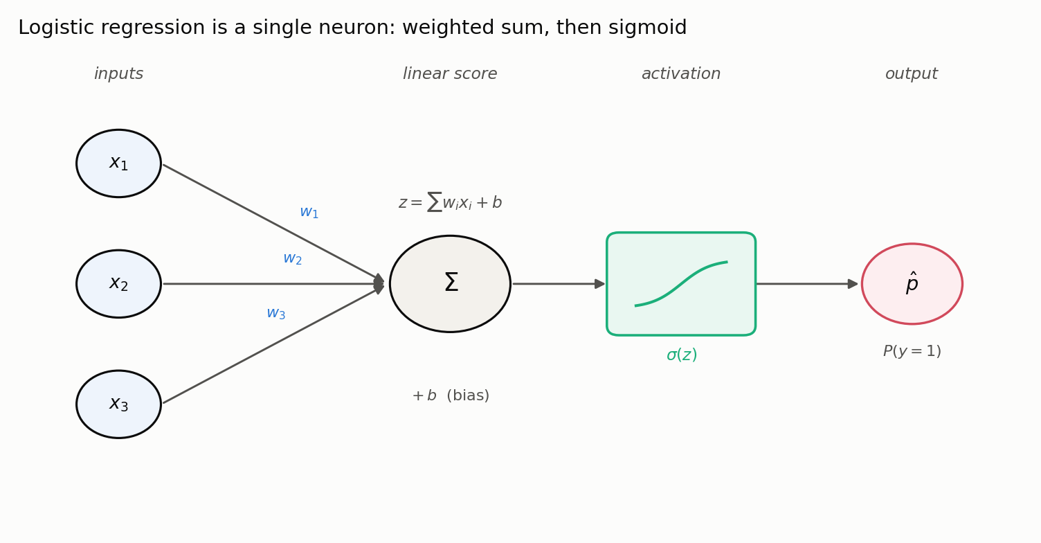
Reading left to right, the neuron does exactly what logistic regression does: it forms the linear score $z = \sum_i w_i x_i + b$, passes it through the sigmoid activation, and emits $\hat p = P(y=1)$. The weights are the coefficients and the bias is the intercept.
Side-by-Side Comparison
Let’s compare the steps and terminology for both:
| Component / Step | Binary Logistic Regression | Single-Neuron Neural Network |
|---|---|---|
| Inputs | A vector of input features X = (x₁, x₂, ...) | The input layer, which takes features X = (x₁, x₂, ...) |
| Processing Step 1: Linear Combination | Calculates a linear score: z = β₀ + β₁x₁ + β₂x₂ + ... | The neuron calculates a weighted sum of its inputs plus a bias: z = (w₁x₁ + w₂x₂ + ...) + b |
| Parameters | Coefficients β₁, β₂, … and an intercept β₀. | Weights w₁, w₂, … and a bias b. (Coefficients are equivalent to weights, and the intercept is the bias). |
| Processing Step 2: Non-Linear Function | Applies the Sigmoid function to the score z to get a probability: P(y=1) = σ(z) | Applies an Activation Function to the weighted sum z. For binary classification, the classic choice is the Sigmoid function. |
| Output | A single value between 0 and 1, representing the probability of the positive class. | A single output value from the neuron, which is interpreted as the probability of the positive class. |
| Loss Function | Binary Cross-Entropy (Log Loss) | Binary Cross-Entropy (the standard loss function for binary classification). |
| Training Method | Gradient Descent (or similar optimizers) to find the β values that minimize the loss. | Gradient Descent (and backpropagation) to find the w and b values that minimize the loss. |
The Key Takeaway
As the table shows, the structure, mathematical operations, and training process are identical. A logistic regression classifier is a neural network in its simplest possible form.
The power and complexity of “deep learning” come from what happens when we start adding more to this simple structure:
- Adding More Neurons: If we add more neurons in the output layer, we can perform multiclass classification (like the Softmax Regression we discussed).
- Adding Hidden Layers: When we stack layers of neurons between the input and output, we create a “deep” neural network. These hidden layers allow the network to learn progressively more complex and abstract patterns from the data, which is something a simple logistic regression model cannot do.
So, understanding logistic regression is a fantastic starting point for understanding neural networks, because a neural network is essentially a collection of these logistic regression-like units, stacked in clever ways to solve much more difficult problems.
2. Extending Logistic Regression Beyond Two Classes
Yes, absolutely!
While the classic form of logistic regression is designed for binary classification (two classes), it can be cleverly extended to handle multiclass classification problems with three or more classes.
There are two primary strategies for doing this:
1. One-vs-Rest (OvR) or One-vs-All (OvA)
This is the most intuitive and common approach. It breaks down the multiclass problem into multiple binary classification problems.
How it works: Imagine a problem with three classes: Cat, Dog, and Bird.
Instead of trying to solve one complex problem, we train three separate binary logistic regression models:
- Model 1 (Cat vs. Not Cat): This model is trained to distinguish
Cat(as the positive class) fromDogandBirdcombined (as the negative class). - Model 2 (Dog vs. Not Dog): This model is trained to distinguish
Dog(positive class) fromCatandBird(negative class). - Model 3 (Bird vs. Not Bird): This model is trained to distinguish
Bird(positive class) fromCatandDog(negative class).
To make a new prediction: When a new image arrives, we run it through all three models. Each model outputs a probability.
- Model 1 might say: “70% probability this is a
Cat.” - Model 2 might say: “15% probability this is a
Dog.” - Model 3 might say: “10% probability this is a
Bird.”
We simply choose the class with the highest probability. In this case, we would classify the image as a Cat.
Because the OvR models are trained independently, their raw positive-class probabilities need not sum to 1. They are primarily competing scores unless the implementation normalizes or calibrates them.
2. Multinomial Logistic Regression (Softmax Regression)
This is a more direct and statistically sophisticated approach. Instead of training multiple independent binary models, we train a single, unified model that is a direct generalization of logistic regression.
How it works: This model uses the Softmax function (which is a generalization of the sigmoid function) as its final step.
- The model calculates a score for each class.
- The Softmax function takes these scores and converts them into a probability distribution, ensuring that the probabilities for all classes add up to 1.
For the same new image, a Multinomial/Softmax model would directly output something like:
- Probability of
Cat: 0.75 - Probability of
Dog: 0.18 - Probability of
Bird: 0.07 - (Total = 1.0)
We again pick the class with the highest probability, which is Cat.
Which one is used in practice?
Current scikit-learn versions optimize multinomial loss for three or more classes when the selected solver supports it. The older multi_class switch has been deprecated. To request One-vs-Rest explicitly, wrap the binary estimator:
1
2
3
4
from sklearn.linear_model import LogisticRegression
from sklearn.multiclass import OneVsRestClassifier

ovr_model = OneVsRestClassifier(LogisticRegression())
Solvers such as lbfgs, newton-cg, newton-cholesky, sag, and saga support multinomial loss, subject to their penalty constraints. The liblinear solver is binary; use the wrapper above when combining it with OvR. Always check the documentation for the installed library version because solver and default behavior can change.
3. Deriving Multinomial Logistic Regression and Softmax
Let’s Assume we’re trying to use multinomial logistic regression to predict whether a person would like one of these three flavours of ice creams: vanilla, chocolate or strawberry. Let’s also assume our independent variables are age, and gender. Here is how the log-odds equations for our ice cream preference model would be structured in multinomial logistic regression.
A key concept in multinomial logistic regression is the use of a reference category. The model calculates the log-odds of an outcome for each category relative to this reference category.
Let’s choose Vanilla as our reference category. This is a common choice, but any of the three could be selected.
Variable Setup
First, we need to define our variables:
- Age: This is a continuous variable, let’s call it
X₁. - Gender: This is a categorical variable. To use it in the model, we need to create a dummy variable. Let’s create
X₂where:X₂ = 1if the person is FemaleX₂ = 0if the person is Male (Male will be the baseline for gender)
The Log-Odds Equations
Since we have 3 classes (Vanilla, Chocolate, Strawberry) and Vanilla is our reference, the model will produce 3 - 1 = 2 log-odds equations.
Each equation will have its own unique set of coefficients (an intercept $\beta_0$, a coefficient for age $\beta_1$, and a coefficient for gender $\beta_2$).
Equation 1: Log-Odds of Preferring Chocolate vs. Vanilla
This equation models the logarithm of the odds that a person prefers Chocolate over Vanilla.
\[\ln\left(\frac{P(\text{Chocolate})}{P(\text{Vanilla})}\right) = \beta_{0, \text{choc}} + \beta_{1, \text{choc}} \cdot (\text{Age}) + \beta_{2, \text{choc}} \cdot (\text{Gender})\]- $\beta_{0, \text{choc}}$ (Intercept): The baseline log-odds of preferring Chocolate over Vanilla for a male (
Gender=0) of age 0. - $\beta_{1, \text{choc}}$ (Age Coefficient): The change in the log-odds of preferring Chocolate over Vanilla for each one-year increase in age, holding gender constant.
- $\beta_{2, \text{choc}}$ (Gender Coefficient): The change in the log-odds of preferring Chocolate over Vanilla if the person is female, compared to being male, holding age constant.
Equation 2: Log-Odds of Preferring Strawberry vs. Vanilla
Similarly, this equation models the logarithm of the odds that a person prefers Strawberry over Vanilla.
\[\ln\left(\frac{P(\text{Strawberry})}{P(\text{Vanilla})}\right) = \beta_{0, \text{straw}} + \beta_{1, \text{straw}} \cdot (\text{Age}) + \beta_{2, \text{straw}} \cdot (\text{Gender})\]- $\beta_{0, \text{straw}}$ (Intercept): The baseline log-odds of preferring Strawberry over Vanilla for a male (
Gender=0) of age 0. - $\beta_{1, \text{straw}}$ (Age Coefficient): The change in the log-odds of preferring Strawberry over Vanilla for each one-year increase in age, holding gender constant.
- $\beta_{2, \text{straw}}$ (Gender Coefficient): The change in the log-odds of preferring Strawberry over Vanilla if the person is female, compared to being male, holding age constant.
Why is there no equation for Vanilla?
There is no equation for the reference category (Vanilla) because the log-odds of preferring Vanilla over Vanilla would be ln(P(Vanilla)/P(Vanilla)) = ln(1) = 0. All effects are measured relative to this baseline. The model uses these two equations along with the constraint that all probabilities must sum to 1 (P(Vanilla) + P(Chocolate) + P(Strawberry) = 1) to calculate the individual probabilities for each of the three flavors.
The Setup
For simplicity, let’s represent the entire linear combination of coefficients and variables with $Z$:
- $Z_{\text{choc}} = \beta_{0, \text{choc}} + \beta_{1, \text{choc}} \cdot (\text{Age}) + \beta_{2, \text{choc}} \cdot (\text{Gender})$
- $Z_{\text{straw}} = \beta_{0, \text{straw}} + \beta_{1, \text{straw}} \cdot (\text{Age}) + \beta_{2, \text{straw}} \cdot (\text{Gender})$
We have two core equations and the fundamental constraint that all probabilities must sum to 1:
- \[\ln\left(\frac{P(\text{Chocolate})}{P(\text{Vanilla})}\right) = Z_{\text{choc}}\]
- \[\ln\left(\frac{P(\text{Strawberry})}{P(\text{Vanilla})}\right) = Z_{\text{straw}}\]
- \[P(\text{Vanilla}) + P(\text{Chocolate}) + P(\text{Strawberry}) = 1\]
Our goal is to isolate P(Chocolate) from these three equations.
Step-by-Step Derivation
Step 1: Exponentiate the log-odds equations to solve for the odds.
We apply the exponential function e to both sides of equations 1 and 2 to remove the natural log ln.
- From equation 1: $P(\text{C})/P(\text{V}) = e^{Z_{\text{choc}}}$
- From equation 2: $P(\text{S})/P(\text{V}) = e^{Z_{\text{straw}}}$
Step 2: Express P(Chocolate) and P(Strawberry) in terms of P(Vanilla).
From the results in Step 1, we can rearrange the terms:
- $P(\text{C}) = P(\text{V}) \times e^{Z_{\text{choc}}}$ (Let’s call this Equation 4)
- $P(\text{S}) = P(\text{V}) \times e^{Z_{\text{straw}}}$ (Let’s call this Equation 5)
This shows that the probabilities of the other categories are proportional to the probability of the reference category, scaled by their respective exponentiated scores.
Step 3: Substitute these into the probability constraint equation.
Now we take our main constraint (Equation 3) and replace P(Chocolate) and P(Strawberry) with what we found in Step 2.
Step 4: Solve for the probability of the reference category, P(Vanilla).
We can factor out P(Vanilla) from the left side of the equation:
Now, divide both sides to isolate P(Vanilla):
Step 5: Derive the final probability for P(Chocolate).
We’re almost there. We go back to Equation 4 from Step 2: $P(\text{C}) = P(\text{V}) \times e^{Z_{\text{choc}}}$ and substitute the expression for P(Vanilla) that we just found in Step 4:
Simplifying this gives our final formula:
\[P(\text{Chocolate}) = \frac{e^{Z_{\text{choc}}}}{1 + e^{Z_{\text{choc}}} + e^{Z_{\text{straw}}}}\]Connection to the Sigmoid Function and Final Softmax Form
This looks very similar to the Softmax formula we discussed earlier. To make the connection perfect, remember that the “score” for our reference category, Vanilla, is implicitly zero.
The log-odds of preferring Vanilla over Vanilla is $\ln(\text{P(V)}/\text{P(V)}) = \ln(1) = 0$. So, we can say $Z_{\text{van}} = 0$.
This means that $e^{Z_{\text{van}}} = e^0 = 1$.
If we substitute $e^{Z_{\text{van}}}$ for the 1 in our denominator, we get the generalized Softmax function:
\[P(\text{Chocolate}) = \frac{e^{Z_{\text{choc}}}}{e^{Z_{\text{van}}} + e^{Z_{\text{choc}}} + e^{Z_{\text{straw}}}}\]This demonstrates that the probability for any given class is the exponentiated score for that class divided by the sum of the exponentiated scores for all possible classes, including the reference category. This is exactly how the sigmoid function is a special case of the softmax function when there are only two classes.
Reference-Class and Full-Score Parameterizations
The derivation above fixes Vanilla’s score to zero, giving an identifiable reference-class parameterization with $K-1$ coefficient vectors. Many machine-learning libraries instead store one score vector for every class and compute:
\[P(Y=k\mid x)=\frac{e^{z_k}}{\sum_{j=1}^{K}e^{z_j}}.\]Both views produce the same kind of probabilities. Adding the same constant to every $z_k$ leaves softmax unchanged, so the full-score parameterization contains a shared-shift redundancy that the reference-class formulation removes.
For numerical stability, implementations evaluate softmax after subtracting the largest score:
\[P(Y=k\mid x) =\frac{e^{z_k-z_{\max}}}{\sum_j e^{z_j-z_{\max}}}.\]This changes neither the probabilities nor the predicted class, but it prevents large exponentials from overflowing.
4. Training and Evaluating with Imbalanced Data
Class imbalance is common, but it does not automatically make logistic regression invalid or useless. The model can still estimate conditional probabilities. The practical difficulties are that minority patterns are supported by fewer observations, accuracy can hide serious errors, and a default 0.5 threshold may not reflect the real cost of mistakes.
Why is an Imbalanced Dataset a Problem?
- The Accuracy Trap: A constant majority-class prediction can achieve 90% accuracy in a 90/10 dataset while never identifying the minority class.
- Limited Minority Evidence: With few minority observations, coefficient estimates for minority-specific patterns can have high variance.
- Decision Costs: The statistically natural threshold is not necessarily the operationally useful threshold. Fraud screening, for example, may tolerate more false positives to capture more true fraud.
The correct response begins with evaluation and decision costs, not automatic resampling.
Strategy 1: Use Appropriate Evaluation Metrics (Absolutely Essential)
Do not use accuracy alone. Choose metrics that reflect the positive class and the relative costs of false positives and false negatives.
- Confusion Matrix: Always start by looking at this. It shows exactly where the model is failing (e.g., a high number of False Negatives, where it predicts “yes” but the answer was “no”).
- Precision and Recall:
- Recall (Sensitivity): Of all the actual “no” cases, how many did the model correctly identify? This is crucial for finding the minority class.
- Precision: Of all the times the model predicted “no”, how many were actually correct? This measures the cost of a false alarm.
- F1-Score: The harmonic mean of precision and recall. It is useful when those two quantities matter similarly, but it ignores true negatives and probability calibration.
- ROC AUC: Measures ranking across thresholds. It can still look strong when the false-positive burden is operationally unacceptable in a highly imbalanced population.
- Precision-Recall (PR) AUC: Focuses on positive-class retrieval. Always compare it with the no-skill baseline, which equals the positive-class prevalence.
- Log loss and calibration: Use these when the probabilities themselves drive decisions rather than only the final labels.
Strategy 2: Use Class Weighting (Easy and Effective)
Class weighting is a useful model-level option when minority mistakes should contribute more to the objective.
How it works: We modify the loss function so that the penalty for misclassifying a “no” sample is much higher than for a “yes” sample. In our 90/10 example, we would give the “no” class a weight of 9 and the “yes” class a weight of 1. This forces the model to work much harder to learn the patterns of the rare class.
Weighting changes the objective, not just the final threshold. As a result, weighted-model probabilities may no longer be calibrated to the natural class prevalence. Evaluate calibration and consider Platt scaling or isotonic calibration on untouched validation data when probability quality matters. If the ranking is already good, tuning the decision threshold may be preferable to refitting with weights.
In Python (scikit-learn): This is incredibly easy to implement. We just set one parameter.
1
2
3
4
5
6
7
8
9
10
from sklearn.linear_model import LogisticRegression

# The 'balanced' mode automatically adjusts weights inversely
# proportional to class frequencies.
model = LogisticRegression(class_weight='balanced')

# Or you can set it manually
# model = LogisticRegression(class_weight={0: 9.0, 1: 1.0}) # Assuming 'no' is 0, 'yes' is 1

model.fit(X_train, y_train)
Strategy 3: Resample the Training Data
This approach involves modifying the training dataset to make it balanced before we feed it to the model.
Resampling must happen only inside the training portion of each split or cross-validation fold. Resampling before the train/test split lets information from synthetic or duplicated observations leak into evaluation.
- Undersampling the Majority Class:
- What it is: Randomly remove samples from the majority class (“yes”) until it’s balanced with the minority class (“no”).
- Pros: Can make training much faster on very large datasets.
- Cons: We might throw away valuable information contained in the majority class samples we discard.
- Oversampling the Minority Class:
- What it is: Randomly duplicate samples from the minority class (“no”) until it’s balanced.
- Pros: Doesn’t lose any data.
- Cons: Can lead to the model overfitting on the specific “no” samples it has seen, as it’s just seeing the same data again and again.
- Synthetic Data Generation (SMOTE):
- What it is: SMOTE (Synthetic Minority Over-sampling Technique) is a smarter way to oversample. Instead of duplicating samples, it creates new, synthetic samples of the minority class. It does this by looking at a “no” sample, finding its nearest “no” neighbors, and creating a new point somewhere along the lines connecting them.
- Trade-off: Can help when local neighborhoods are meaningful, but can also create unrealistic points, blur class boundaries, and behave poorly with sparse or high-dimensional features. It must be validated rather than assumed superior.
Recommended Workflow
- Split first: Create stratified training, validation, and test partitions before weighting or resampling.
- Define the error costs: Decide whether false positives, false negatives, ranking, or calibrated probabilities matter most.
- Build an unmodified baseline: Report the confusion matrix, precision, recall, PR-AUC with its prevalence baseline, ROC-AUC, and calibration as appropriate.
- Tune the threshold: Choose it on validation data using the real cost or capacity constraint, not the test set.
- Compare interventions: Evaluate class weighting, undersampling, oversampling, or SMOTE separately inside training folds.
- Check calibration: If probabilities drive decisions, calibrate using held-out data after selecting the model.
- Evaluate once on the untouched test set: Report uncertainty and the final operating threshold.
Do not combine class weighting and SMOTE by default. They both alter the effective class distribution, and their combination can overcorrect. Let cross-validation against the real objective decide.
Closing Perspective
Logistic regression is a compact bridge between statistics and machine learning. Its coefficients support statistical interpretation, its sigmoid and softmax outputs support probabilistic classification, its loss connects directly to likelihood, and its architecture reappears as the output layer of neural networks.
Across the three parts, we moved from how the binary model is trained, through what its coefficients and boundary mean, to how the same ideas extend to multiclass and imbalanced settings.