Linear Regression, Part 2: Multicollinearity and Regularization
Diagnose multicollinearity and understand how Ridge, Lasso, Elastic Net, and Bayesian priors stabilize or simplify linear regression.
- OLS foundations
- Multicollinearity and regularization You are here
- Evaluation and interpretation
- Bayesian linear regression
- From log-odds to gradient descent
- Coefficients and decision boundaries
- Softmax and imbalanced data
In Part 1 we derived the OLS solution and saw that it relies on a stable, invertible $X^T X$. Correlated features attack exactly that requirement: they make coefficient estimates unstable and can make the normal equation singular.
This part traces the problem from diagnosis to treatment. We will measure multicollinearity with VIF, explain why coefficients can explode, and compare the different behaviors of Ridge, Lasso, and Elastic Net. We will then connect those penalties to their Bayesian interpretation.
1. Understanding Multicollinearity and VIF
The Problem: What is Multicollinearity?
Multicollinearity is when two or more of the independent features (X variables) are highly correlated with each other.
Analogy: Suppose we are trying to predict house_price with two features: temperature_in_celsius and temperature_in_fahrenheit. They are perfectly correlated! If we include both, the model has no idea how to assign “importance.” Should it give all the weight to Celsius? Or Fahrenheit? Or split it 50/50?
This makes the model’s coefficients (the “weights”) unstable and their p-values unreliable. Our model might say temperature_in_celsius is “not significant” simply because all its predictive power is also “explained” by temperature_in_fahrenheit.
The Solution: VIF (Variance Inflation Factor)
VIF is a diagnostic tool used to measure how much multicollinearity exists for a specific feature.
- It’s a score calculated for each independent feature in our model.
- The score shows how much the variance of that feature’s coefficient is “inflated” (increased) due to its correlation with other features.
How VIF is Calculated (The 4-Feature Example)
This is the most important part to explain. VIF is calculated by running a “mini” linear regression inside the main regression.
Let’s use an example:
- Target (y):
fraud_amount - Features (X):
X1:transaction_amountX2:user_ageX3:num_transactions_past_24hX4:total_value_past_24h(This will be our problem-child)
The problem is that X4 (total_value_past_24h) is almost certainly going to be highly correlated with X1 (transaction_amount) and X3 (num_transactions_past_24h).
To calculate the VIF for feature X4, we do the following:
- Isolate
X4: Temporarily removeX4from the “feature” list and make it the new target. - Run a New Regression: Run a new linear regression model where we try to predict
X4using all other features:X4 ~ X1 + X2 + X3 - Get the R-squared: Look at the
R^2of this new model. ThisR^2tells us how well the other features can explainX4.- Since
X1andX3are very predictive ofX4, thisR^2will be very high. Let’s say it’s 0.98. This means 98% of the variance inX4is already explained by the other features.
- Since
- Calculate VIF: The formula is:
VIF = 1 / (1 - R^2)- For
X4:VIF = 1 / (1 - 0.98) = 1 / 0.02 = 50
- For
Now, let’s do the same for a “good” feature, X2 (user_age):
- Isolate
X2: MakeX2the target. - Run Regression:
X2 ~ X1 + X3 + X4 - Get the R-squared: How well can transaction amounts predict a user’s age? Probably not very well. The
R^2will be very low, maybe 0.1. - Calculate VIF:
- For
X2:VIF = 1 / (1 - 0.1) = 1 / 0.9 = 1.11
- For
How to Interpret and Use the VIF Scores (The Action Plan)
This is how we use the scores to remove the dependent variables.
Rules of Thumb for VIF Scores:
- VIF = 1: Not correlated at all (perfectly independent).
- VIF < 5: Generally considered acceptable.
- VIF > 5 (or > 10): Highly correlated. This feature is a problem and needs to be addressed. (The 5 or 10 threshold is a matter of preference, 5 is more strict).
The Action Plan (An Iterative Process):
This is the most critical part of the answer. We do not remove all features with VIF > 5 at the same time.
- Run VIF for all features:
VIF(X1)= 4.5VIF(X2)= 1.11VIF(X3)= 4.8VIF(X4)= 50.0
- Find the Highest VIF: The highest VIF is
X4(50.0). It is well above our threshold of 5. - Remove only that one feature. Remove
X4(total_value_past_24h) from the model. - Re-run VIF: Now, we must re-calculate the VIFs for the remaining features (
X1,X2,X3).- Why? Because
X1andX3were correlated withX4. Now thatX4is gone, their VIFs might have dropped. - New VIFs:
VIF(X1)= 1.5VIF(X2)= 1.10VIF(X3)= 1.4
- Why? Because
- Check Again: All VIFs are now well below 5. The multicollinearity is fixed. We can now proceed to build the final linear regression model with features
X1,X2, andX3.
This iterative removal process is the standard, robust way to use VIF to remove linearly dependent variables.
2. Why OLS Coefficients Explode - and How Ridge Responds
To understand how L2 regularization (Ridge) fixes multicollinearity, we first need to understand why multicollinearity breaks standard Linear Regression (Ordinary Least Squares - OLS).
1. The Problem: Why OLS Breaks with Multicollinearity
Imagine we are trying to predict House Price ($y$) with two features that are almost identical:
- $x_1$: Size in Square Feet
- $x_2$: Size in Square Meters
Obviously, these two are perfectly correlated. They contain the exact same information.
The “Exploding Coefficients” Phenomenon: In standard OLS, the model tries to minimize error. It doesn’t care about the size of the coefficients (weights). If the true relationship is $y = 1 \cdot x_1$ (Price = 1 * SqFt), the model has infinite ways to express this using both features:
- $1 \cdot x_1 + 0 \cdot x_2$ (Correct)
- $0 \cdot x_1 + 10.76 \cdot x_2$ (Correct)
- $1001 \cdot x_1 - 10760 \cdot x_2$ (Also mathematically “correct” on training data!)
With multicollinearity, nothing in the OLS objective rules the third option out - all three fit the training data equally well. Which one we actually get is a property of the solver and the noise in the data, not of OLS preferring extremes; section 4 below makes that precise. What is unambiguously true is that the fitted coefficients become unstable (high variance): a tiny bit of noise can swing them wildly, including into huge canceling pairs.
2. The Intuitive Fix: L2 Penalizes “Heroes and Villains”
L2 Regularization adds a penalty term to the loss function: $\lambda \sum \beta^2$.
It forces the model to minimize the sum of squares of the weights.
Let’s look at our previous example weights under the L2 lens:
- Option A (Balanced): $\beta_1 = 0.5, \beta_2 \approx 5.3$
- L2 Penalty $\approx 0.5^2 + 5.3^2 \approx \mathbf{28}$
- Option B (Wild): $\beta_1 = 1001, \beta_2 = -10760$
- L2 Penalty $\approx 1001^2 + (-10760)^2 \approx \mathbf{116,000,000}$
The Result: The L2 penalty makes Option B astronomically expensive. The optimization algorithm will aggressively reject those massive canceling weights.
Instead, L2 regularization encourages the model to share the credit. It pushes the coefficients toward a stable, balanced distribution where correlated features share the weight, rather than one taking a massive positive value and the other a massive negative value.
3. The Infinite Family of Solutions
With perfect multicollinearity (or near-perfect multicollinearity), the model moves from having one unique optimal solution to having an infinite family of equally good solutions.
In our example, $x_2$ (Square Meters) is just $x_1$ (Square Feet) times a constant $C \approx 10.76$.
The target is to minimize the loss (MSE):
\[\text{Loss} = \sum (y - (\beta_1 x_1 + \beta_2 x_2 + \beta_0))^2\]Since $x_2 \approx 0.093 x_1$, the term $(\beta_1 x_1 + \beta_2 x_2)$ can be rewritten:
\[(\beta_1 + \beta_2 \cdot 0.093) x_1\]The model only cares about the sum $\beta_1 + \beta_2 \cdot 0.093$. Any pair of weights that gives the required final sum will result in the exact same minimal loss.
| Option | $\beta_1$ | $\beta_2$ | Final Combination (The Sum) | Loss (MSE) |
|---|---|---|---|---|
| 1 | 1.0 | 0.0 | $\approx 1.0$ | Minimum |
| 2 | 0.0 | 10.76 | $\approx 1.0$ | Minimum |
| 3 | 1001.0 | -10760.0 | $\approx 1.0$ | Minimum |
Since all three options result in the same minimum error (the same altitude), the optimizer has no mathematical reason to prefer Option 1 or 2 over Option 3.
4. Where the Exploding Coefficients Actually Come From
The flat valley explains why the danger exists. Solver behavior decides where in the valley we land - and the two collinearity regimes behave differently:
- Perfect multicollinearity (exact duplicates): the solution is genuinely non-unique - the valley floor is exactly flat. But standard solvers do not wander to a random corner of it. A pseudoinverse-based solver (
numpy.linalg.pinv,lstsq) returns the minimum-norm solution: the smallest point in the valley, not an exploding one. Gradient descent initialized at zero has the same implicit bias - its updates never leave the row space of $X$, so it converges to the minimum-norm solution too. The cartoon of OLS “choosing” 1001 and -10760 does not come from this case. - Near multicollinearity (the realistic case): the solution is unique - but the unique minimum is defined by tiny differences between almost-redundant columns. This is ill-conditioning: the answer exists but is exquisitely sensitive to noise. Small perturbations in the data slide the unique minimum enormous distances along the nearly-flat valley floor, and this is where the huge, opposite-signed coefficient pairs genuinely appear. Refit on a slightly different sample and the pair reshuffles completely.
Conclusion:
The honest summary is not “OLS prefers extreme weights.” It is: under near-collinearity the estimate is unique yet so ill-conditioned that the noise effectively chooses it - and noise has no taste for small coefficients.
L2 Regularization solves this by adding a “hill” to the flat valley. It tells the optimizer to also minimize the size of the weights. This forces the optimizer to the center of the flat valley, where the weights are smallest (Option 1 or 2), thus fixing the instability.
3. Why $X^T X + \lambda I$ Is Invertible
The guarantee that $(X^T X + \lambda I)$ is invertible lies in the mathematical properties of the matrices and the effect that adding a scaled identity matrix has on them. The explanation involves a few key concepts from linear algebra, primarily focused on eigenvalues.
Here is the step-by-step reasoning:
Step 1: Understanding the Properties of $X^T X$
The matrix $X^T X$ has a special property: it is positive semi-definite. Let’s break down what this means.
- Definition: A matrix $A$ is positive semi-definite if for any non-zero vector $v$, the scalar result of the quadratic form $v^T A v$ is non-negative (i.e., $v^T A v \ge 0$).
Proof for $X^T X$: Let’s apply this to our matrix. For any non-zero vector $v$:
\[v^T (X^T X) v = (Xv)^T (Xv)\]This can be rewritten using the definition of the Euclidean norm (or length) of a vector, which is:
\[\lVert z \rVert^2 = z^T.z\] \[(Xv)^T (Xv) = \lVert Xv \rVert^2\]The squared norm (or length) of any vector is always greater than or equal to zero. Therefore, $v^T (X^T X) v \ge 0$, which proves that $X^T X$ is positive semi-definite.
Step 2: The Link Between Invertibility and Eigenvalues
A fundamental theorem in linear algebra states:
A square matrix is invertible if and only if all of its eigenvalues are non-zero.
If a matrix has at least one eigenvalue equal to zero, it is singular (not invertible). So, the entire problem of $X^T X$ being non-invertible is that it has at least one eigenvalue of 0.
Step 3: Eigenvalues of a Positive Semi-Definite Matrix
A key property that follows from the definition in Step 1 is that all eigenvalues of a positive semi-definite matrix are non-negative.
So, for our matrix $X^T X$, if we call its eigenvalues $\mu_i$, then we know that:
\[\mu_i \ge 0 \quad \text{for all } i\]If $X^T X$ is not invertible, it means at least one of these eigenvalues, say $\mu_k$, is exactly 0.
Step 4: The Effect of Adding $\lambda I$
This is the most critical step. Let’s see what happens to the eigenvalues of a matrix when we add a scaled identity matrix ($\lambda I$).
Let $A$ be any square matrix with an eigenvalue $\mu$ and a corresponding eigenvector $v$. By definition, this means:
\[Av = \mu v\]Now, let’s look at our new regularized matrix, $B = A + \lambda I$. What happens when we multiply it by the same eigenvector $v$?
\[Bv = (A + \lambda I)v\] \[Bv = Av + \lambda I v\] \[Bv = Av + \lambda v\]Since we know $Av = \mu v$, we can substitute it back in:
\[Bv = \mu v + \lambda v\] \[Bv = (\mu + \lambda)v\]This final equation, $Bv = (\mu + \lambda)v$, shows that $v$ is also an eigenvector of the new matrix $B$, but its corresponding eigenvalue is now $(\mu + \lambda)$.
Conclusion: Putting It All Together
We can now connect all the pieces to see why $(X^T X + \lambda I)$ is always invertible:
- The eigenvalues of $X^T X$ are all greater than or equal to zero ($\mu_i \ge 0$).
- The regularization parameter $\lambda$ is always chosen to be a small, strictly positive number ($\lambda > 0$).
From Step 4, we know that the eigenvalues of the new matrix $(X^T X + \lambda I)$ are simply the original eigenvalues plus $\lambda$. Let’s call the new eigenvalues $\mu’_i$.
\[\mu'_i = \mu_i + \lambda\]Since $\mu_i \ge 0$ and $\lambda > 0$, their sum must be strictly positive:
\[\mu'_i > 0\]
This proves that every eigenvalue of the regularized matrix $(X^T X + \lambda I)$ is strictly positive. Since none of its eigenvalues can be zero, the matrix is guaranteed to be invertible.
In essence, the addition of the “ridge” term $\lambda I$ pushes every eigenvalue (including any that were zero) into the positive part of the number line, thereby resolving the singularity problem.
4. Why Lasso Has No Normal Equation
The straightforward answer is: Lasso regression does not have a “normal equation” in the way that Ordinary Least Squares or Ridge Regression do. There is no simple, closed-form analytical solution to find the optimal coefficients.
Let’s break down why this is the case and how Lasso models are solved instead.
1. The Cost Function for Lasso Regression
First, let’s look at the cost function that Lasso regression tries to minimize. It’s the standard Sum of Squared Errors (SSE) plus a penalty term based on the sum of the absolute values of the coefficients (the L1 norm).
\[J_{LASSO}(\beta) = \underbrace{\frac{1}{2m} (X\beta - y)^T(X\beta - y)}_{\text{Sum of Squared Errors}} + \underbrace{\lambda \sum_{j=1}^{n} |\beta_j|}_{\text{L1 Penalty Term}}\]Here, $\lambda$ is the regularization parameter that controls the strength of the penalty.
2. The Problem with Finding a Normal Equation
To find a normal equation, we need to take the derivative (gradient) of the cost function with respect to $\beta$ and set it to zero.
Let’s try that:
\[\nabla_\beta J_{LASSO}(\beta) = \nabla_\beta \left( \frac{1}{2m} (X\beta - y)^T(X\beta - y) \right) + \nabla_\beta \left( \lambda \sum_{j=1}^{n} |\beta_j| \right)\]- The derivative of the first term is the same as in ordinary linear regression: $\frac{1}{m}(X^T X \beta - X^T y)$
- The derivative of the second term is where the problem lies. We need the derivative of the absolute value function, $\lvert x \rvert$.
The derivative of $|x|$ is:
- $1$ if $x > 0$
- $-1$ if $x < 0$
- Undefined at $x = 0$
This derivative is often written as the signum function, $\text{sgn}(x)$.
So, the gradient of the L1 penalty term is $\lambda \cdot \text{sgn}(\beta)$. When we try to set the full gradient to zero, we get:
\[\frac{1}{m}(X^T X \beta - X^T y) + \lambda \cdot \text{sgn}(\beta) = 0\]Rearranging this gives us a pseudo-normal equation:
\[X^T X \beta = X^T y - m\lambda \cdot \text{sgn}(\beta)\]This equation cannot be solved analytically for $\beta$ for two key reasons:
- The $\text{sgn}(\beta)$ term depends on the sign of $\beta$ itself. To solve for $\beta$, we would already need to know its sign, which creates a circular dependency. We can’t isolate $\beta$ on one side of the equation.
- The derivative is undefined when any coefficient $\beta_j = 0$. This is a critical issue because the primary purpose and effect of Lasso regression is to force some coefficients to be exactly zero. The very points we are most interested in are the points where the function is not differentiable.
Because of this non-differentiable nature of the L1 penalty, there is no closed-form solution like a normal equation.
The same non-differentiable corner has a geometric reading that explains why Lasso zeroes coefficients while Ridge merely shrinks them. Picture the elliptical SSE contours around the OLS optimum, and the constraint region the penalty imposes: a diamond for L1, a circle for L2. The solution is where the smallest contour first touches the constraint.
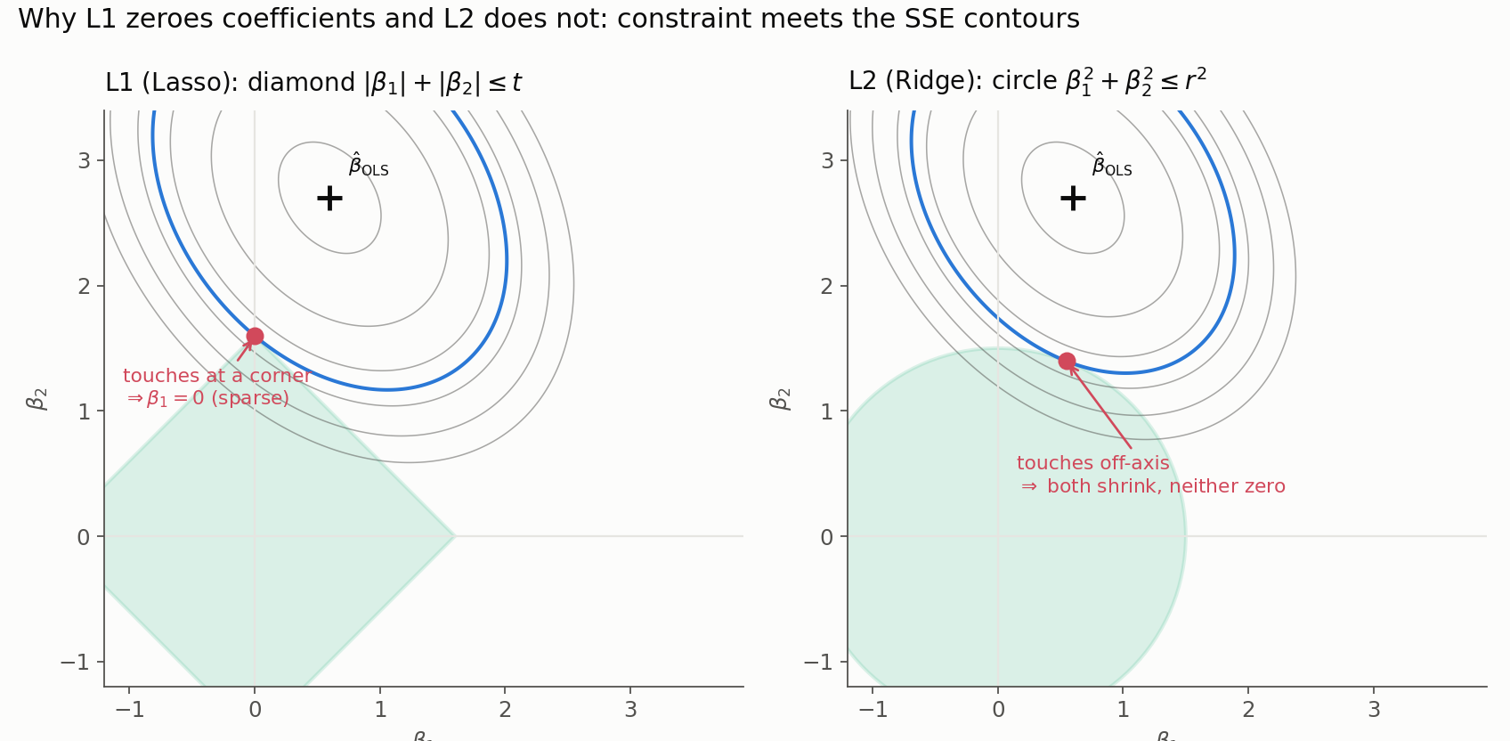
The diamond has its vertices on the axes, so a growing contour tends to strike it at a corner - and a corner sets one coefficient to exactly zero. The circle has no corners, so the contour meets it at a generic point where both coefficients are shrunk but neither vanishes. That single difference in the shape of the constraint is the geometric root of L1’s sparsity.
Two qualifications sharpen that statement. First, “no closed form” means no general normal-equation-style formula for an arbitrary design matrix. Special cases do have one: with an orthonormal design ($X^T X = I$), the Lasso solution is exactly OLS followed by soft-thresholding - shrink each OLS coefficient toward zero by the penalty amount, and set to zero any coefficient the shrinkage crosses. Second, the “pseudo-normal equation” above is more useful than it looks. Read as a subgradient (KKT) condition, it says a coefficient can sit exactly at zero whenever its feature’s correlation with the residual is smaller than the penalty strength - which is simultaneously why Lasso produces exact zeros and why coordinate descent works: each coordinate update is that one-dimensional soft-threshold applied in turn.
Contrast with Ridge Regression (L2)
It’s helpful to contrast this with Ridge Regression, which uses an L2 penalty ($\lambda \sum \beta_j^2$). The derivative of $\beta_j^2$ is simply $2\beta_j$. This is a well-behaved linear function, which leads to the clean, solvable normal equation we saw earlier:
\[X^T X \beta + \lambda I \beta = X^T y \implies \hat{\beta} = (X^T X + \lambda I)^{-1} X^T y\]So, How Is Lasso Solved?
Since there is no analytical solution, Lasso regression must be solved using iterative numerical optimization algorithms. These algorithms can handle the non-differentiable point at zero and can converge to the optimal solution.
Common methods include:
- Coordinate Descent: This is the most popular and often most efficient method for Lasso. It works by optimizing one coefficient at a time, holding all others fixed, and cycling through all the coefficients repeatedly until the solution converges.
- Subgradient Methods: These are a generalization of gradient descent that can be used for non-differentiable functions. Instead of a gradient, they use a “subgradient,” which provides a direction for the update.
- Least Angle Regression (LARS): This is a clever and efficient algorithm that is closely related to Lasso. In some cases, it can compute the entire path of Lasso solutions for every possible value of $\lambda$.
5. Lasso vs. Ridge for Correlated Features
L1 (Lasso) regularization does address multicollinearity by forcing coefficients to zero, effectively performing feature selection.
However, it is often not the preferred mechanism because of how it solves it. Its solution is arbitrary and unstable in a way that L2 (Ridge) is not.
Here is why L2 is generally preferred for multicollinearity unless we explicitly want feature selection.
1. The Arbitrary Selection Problem
Imagine we have two identical features: $x_1$ (Height in cm) and $x_2$ (Height in inches). They are perfectly correlated.
- L2 (Ridge): With the features standardized to a common scale, Ridge assigns them roughly equal weights ($\beta_1 \approx \beta_2$) - the grouping effect. (On raw units the split follows the scale difference instead, so standardize before reading coefficients this way.)
- Result: The model says “Both of these height features are important.” It uses the information from both. This is stable. If we run the training again, we get the same result.
- L1 (Lasso): Will arbitrarily pick one and kill the other.
- Result: It might set $\beta_1 = \text{high}, \beta_2 = 0$.
- The Problem: Which one does it pick? The choice is arbitrary and unstable rather than literally random: for fixed data and settings, most solvers are deterministic - but the winner can hinge on incidental details like column order or floating-point noise, and with perfectly correlated features the Lasso optimum is not even unique.
- Instability: If we slightly perturb the data or retrain the model, Lasso might suddenly flip and pick $x_2$ instead of $x_1$. This makes the model unstable and confusing to interpret (“Why did ‘Height in Inches’ suddenly become important instead of ‘Height in cm’?”).
2. The “Information Loss” Problem
Multicollinearity often involves features that are highly correlated but not identical.
- Example: $x_1$ = “Minutes played in first half”, $x_2$ = “Minutes played in second half” for a soccer player. These are highly correlated (good players play more).
- L2 (Ridge): Keeps both. It allows both features to contribute their unique signal to the prediction.
- L1 (Lasso): Might see them as redundant and drop one entirely (e.g., set weight of $x_2$ to 0).
- Consequence: We have lost the unique information contained in $x_2$. The model is simpler, but potentially less accurate.
Summary: When to Use Which
| Feature | L2 (Ridge) | L1 (Lasso) |
|---|---|---|
| Multicollinearity Solution | Shrinks coefficients together. Correlated features share the weight. | Selects one feature arbitrarily and sets others to zero. |
| Stability | Stable. Small data changes lead to small coefficient changes. | Unstable. Small data changes can cause the selected feature to flip completely. |
| Goal | Prediction Accuracy. Keeps all signals, even redundant ones. | Model Simplicity / Feature Selection. Removes redundancy aggressively. |
| Preferred When… | We want the best predictive performance and care about stability. | We have thousands of features and need to filter out the noise (sparse solution). |
Conclusion: L2 is preferred because it handles multicollinearity gracefully by smoothing the impact across correlated variables, whereas L1 handles it abruptly by deleting variables, often arbitrarily.
6. Elastic Net: Combining L1 and L2
Elastic Net is a powerful and popular regularized regression technique in machine learning that effectively combines the strengths of two other regularization methods: Lasso (L1) and Ridge (L2).
Think of it as a hybrid model that gets the “best of both worlds.”
The Core Idea: Solving the Problems of Lasso and Ridge
To understand why Elastic Net was created, let’s look at the limitations of its predecessors:
Ridge Regression (L2 Penalty): This method is excellent at handling multicollinearity (when features are highly correlated). It shrinks the coefficients of correlated features towards each other, without setting any of them to exactly zero. Its main drawback is that it doesn’t perform feature selection. In a model with many irrelevant features, Ridge will keep all of them, making the final model less interpretable.
Lasso Regression (L1 Penalty): This method is great for feature selection. It forces the coefficients of the least important features to become exactly zero, effectively removing them from the model. However, Lasso has a significant drawback: if a group of features are highly correlated, it tends to arbitrarily select only one of them and set the others to zero. This can lead to a loss of information and model instability.
Elastic Net was designed to overcome these limitations by combining both penalties.
The Mathematical Formulation
The cost function for Elastic Net is a simple combination of the cost functions for Lasso and Ridge:
\[J_{ElasticNet}(\beta) = \text{MSE} + \alpha \rho \sum_{j=1}^{n} |\beta_j| + \frac{\alpha(1-\rho)}{2} \sum_{j=1}^{n} \beta_j^2\]Let’s break down this formula:
- MSE: This is the standard Mean Squared Error term, which measures the model’s prediction error.
- The L1 (Lasso) Part: $\alpha \rho \sum_{j=1}^{n} \lvert \beta_j \rvert$
- The L2 (Ridge) Part: $\frac{\alpha(1-\rho)}{2} \sum_{j=1}^{n} \beta_j^2$
The model is controlled by two key hyperparameters:
- $\alpha$ (alpha): This is the overall regularization strength. It controls how much the model is penalized for having large coefficients. A larger $\alpha$ results in more shrinkage.
- $\rho$ (rho) or
l1_ratio: This is the mixing parameter that balances the L1 and L2 penalties. It ranges from 0 to 1.- When $\rho = 1$, the L2 part of the penalty becomes zero, and the model is equivalent to Lasso Regression.
- When $\rho = 0$, the L1 part of the penalty becomes zero, and the model is equivalent to Ridge Regression.
- When $0 < \rho < 1$, the model is a hybrid of the two.
The Advantages of Elastic Net
By combining the two penalties, Elastic Net gains two key advantages:
- Performs Feature Selection like Lasso: The L1 component of the penalty allows Elastic Net to shrink some coefficients to exactly zero, thus removing irrelevant features and creating a more interpretable model.
- Handles Correlated Features like Ridge: The L2 component allows the model to handle multicollinearity effectively. Instead of arbitrarily picking one feature from a highly correlated group (like Lasso might), Elastic Net tends to select the entire group of correlated features, shrinking their coefficients together. This is known as the grouping effect.
When Should We Use Elastic Net?
Elastic Net is a particularly good choice in the following scenarios:
- When we have a large number of features, especially if the number of features is greater than the number of data points.
- When we have highly correlated features (multicollinearity).
- When we are unsure whether Lasso or Ridge would be a better choice. Elastic Net provides a robust alternative that often performs better than either one on its own, and we can use techniques like cross-validation to find the optimal mix of L1 and L2 penalties.
In summary, Elastic Net is a flexible and powerful regularization technique that combines the feature selection capabilities of Lasso with the stability of Ridge when dealing with correlated data, making it a go-to choice for many regression problems.
7. The Bayesian Connection to L1 and L2
This is one of the most elegant connections in machine learning. It bridges the gap between frequentist/optimization approaches (minimizing a loss function) and Bayesian/probabilistic approaches (updating beliefs).
The connection is this: Regularized Linear Regression is exactly equivalent to finding the Maximum A Posteriori (MAP) estimate in a Bayesian Linear Regression model with specific priors.
- Ridge Regression (L2) $\iff$ Bayesian Regression with a Gaussian Prior.
- Lasso Regression (L1) $\iff$ Bayesian Regression with a Laplace Prior.
Let’s break down the math and the intuition to see exactly how this works.
1. The Foundation: Bayes’ Theorem
In Bayesian inference, we update our beliefs about the coefficients ($\beta$) based on the data ($X, y$).
\[P(\beta \vert X, y) = \frac{P(y \vert X, \beta) \cdot P(\beta)}{P(y \vert X)}\]- Posterior: $P(\beta \vert X, y)$ : Our updated belief about the weights after seeing data.
- Likelihood $P(y \vert X, \beta)$ : How well the weights explain the data. Maximizing this is just standard OLS.
- Prior $P(\beta)$ : Our belief about the weights before seeing any data.
- Marginal Likelihood $P(y \vert X)$ : A constant normalization factor (we can ignore this for optimization).
So, finding the best weights ($\beta_{MAP}$) means maximizing:
\[\text{Posterior} \propto \text{Likelihood} \times \text{Prior}\]Or, taking the logarithm (which turns multiplication into addition):
\[\log(\text{Posterior}) \propto \log(\text{Likelihood}) + \log(\text{Prior})\]2. The Connection to L2 (Ridge Regression)
In Ridge regression, we add a penalty term $\lambda \sum \beta_j^2$. Let’s see how this emerges from the Bayesian view.
The Prior: Assume the coefficients come from a Gaussian (Normal) Distribution centered at zero. This means we believe, prior to seeing data, that the weights are likely small and close to zero.
\[P(\beta) = \frac{1}{\sqrt{2\pi\tau^2}} \exp\left( - \frac{\beta^2}{2\tau^2} \right) \Rightarrow P(\beta) \propto \exp\left(-\frac{\beta^2}{2\tau^2}\right)\]What is $\tau$ (tau)?
- $\tau$ is the Standard Deviation of the Gaussian prior.
- It represents our “uncertainty” or “tolerance” for how large the weights can be.
- Large $\tau$: The bell curve is wide and flat. We are okay with large weights. (Weak regularization).
- Small $\tau$: The bell curve is narrow and spiked. We strictly believe weights should be close to zero. (Strong regularization).
The Math: When we calculate the $\log(\text{Posterior})$:
- Log-Likelihood: Becomes the negative sum of squared errors (standard OLS part): $-\sum(y - X\beta)^2$.
- We assume the noise ($\epsilon$) in the data generation process is Gaussian.
- This means $y_i$ follows a Gaussian distribution centered at $\hat{y}_i$.
- This gives us the formula: $\text{Likelihood} \propto \exp(-(y - \hat{y})^2)$.
- This leads to the Mean Squared Error (MSE) term.
- Log-Prior: $\log(\exp(-\beta^2)) = -\beta^2$.
Therefore, maximizing the posterior is equivalent to minimizing:
\[J(\beta) = \sum(y - \hat{y})^2 + \lambda \sum \beta^2\]Conclusion: Ridge Regression is simply Bayesian Regression where we assume the weights are normally distributed. The regularization parameter $\lambda$ is inversely related to the variance of that Gaussian prior.
3. The Connection to L1 (Lasso Regression)
In Lasso regression, we add a penalty term $\lambda \sum \lvert \beta_j \rvert$.
The Prior: Assume the coefficients come from a Laplace Distribution centered at zero. The Laplace distribution looks like a double exponential. Unlike the bell curve (Gaussian), it has a very sharp peak at zero and wider tails.
\[P(\beta) = \frac{1}{2b} \exp\left( - \frac{|\beta|}{b} \right) \Rightarrow P(\beta) \propto \exp\left(-\frac{|\beta|}{b}\right)\]What is $b$?
- $b$ is the Scale Parameter of the Laplace distribution (similar concept to standard deviation).
- It controls how quickly the probability drops off as we move away from zero.
- Large $b$: The peak at zero is dull, and tails are wide. (Weak regularization).
- Small $b$: The peak at zero is extremely sharp. We strongly believe weights should be exactly zero. (Strong regularization).
The Math: When we calculate the $\log(\text{Posterior})$:
- Log-Likelihood: Still the negative sum of squared errors: $-\sum(y - X\beta)^2$.
- Same reason as L2 regularization, since the noise ($\epsilon$) in the data generation process is Gaussian.
- Log-Prior: $\log(\exp(-\lvert \beta \rvert)) = -\lvert \beta \rvert$.
Therefore, maximizing the posterior is equivalent to minimizing:
\[J(\beta) = \sum(y - \hat{y})^2 + \lambda \sum |\beta|\]Conclusion: Lasso Regression is simply Bayesian Regression where we assume the weights follow a Laplace distribution.
4. Why Intuition Matches Reality
This probabilistic view explains the behavior we see in these models:
- Gaussian Prior (Ridge): The Gaussian log-prior is smooth at zero - the penalty $\beta^2$ has zero slope there, so the pull toward zero fades away as a coefficient gets small. Large weights get shrunk, but nothing forces them exactly to zero. This matches Ridge’s behavior: shrinkage, no feature selection.
- Laplace Prior (Lasso): One subtlety matters here: a continuous Laplace prior puts zero probability mass on any exact point, including zero. What it has at zero is a high density with a sharp cusp. The exact zeros come from the optimization, not the prior: the $\lvert \beta \rvert$ penalty is non-differentiable at zero with constant slope on either side, so whenever a coefficient’s evidence from the data is weaker than that slope, the MAP optimum sits exactly at zero. Sparsity is a property of the $L_1$ geometry of the MAP problem - not of the prior “storing” probability at zero.
For the record, the equivalence in this section rests on stated assumptions and one convention: Gaussian observation noise (which makes the log-likelihood the squared error), a zero-mean Gaussian coefficient prior for the $L_2$ penalty, and a zero-mean Laplace coefficient prior for the $L_1$ penalty. The exact mapping between $\lambda$, the noise variance $\sigma^2$, and the prior scale ($\tau$ or $b$) depends on how the loss is normalized (summed or averaged, with or without the $\frac{1}{2}$) - so match conventions before comparing formulas across textbooks or libraries.
Summary Table
| Regression Type | Bayesian Equivalent | Prior Distribution | Why it works? |
|---|---|---|---|
| OLS (Vanilla) | Maximize Likelihood (MLE) | Uniform / Flat (No prior belief) | We assume all weight values are equally probable before seeing data. |
| Ridge (L2) | Maximize Posterior (MAP) | Gaussian (Normal) | We assume weights are likely small and distributed normally around zero. |
| Lasso (L1) | Maximize Posterior (MAP) | Laplace | We assume weights are likely to be exactly zero (sparsity). |
Resources
- What is Multicollinearity? Extensive video + simulation!
- Variance Inflation Factor Simplified
- Bayesian Linear Regression: Data Science Concepts
Regularization tells us how to stabilize or simplify a fitted model. Part 3 turns to the questions that follow training: how well the model performs, how its coefficients should be interpreted, how outliers affect it, and when the linear-regression framework needs to be extended.