Slope and Curvature: A Practical Guide to the Jacobian and Hessian
- Jacobians and Hessians You are here
- Activation functions
- Backpropagation and optimizers
- Initialization and layer normalization
- Regularization
- From SVD to Word2Vec
- RNNs, LSTMs, and GRUs
Most of machine learning runs on first-order information: the gradient tells us which way is downhill, and we take a step. That is enough to train enormous models. But a whole family of methods, from Newton’s method to the second-order model-compression algorithms like GPTQ, lean on something the gradient cannot tell us: how the slope itself changes as we move. That is curvature, and its bookkeeping device is the Hessian.
This is a compact, self-contained primer on the two objects that capture slope and curvature: the Jacobian (first derivatives) and the Hessian (second derivatives). We build them up from definitions, give them a geometric reading, and then show the two places they earn their keep in ML: reasoning about the shape of a loss surface, and the least-squares identity that connects the two. It is written as a reference to link back to whenever a “Hessian” shows up and the intuition has gone fuzzy.
1. First derivatives: the Jacobian
For a vector-valued function $f : \mathbb{R}^n \to \mathbb{R}^m$, the Jacobian is the $m \times n$ matrix of all first partial derivatives:
\[J_{ij} = \frac{\partial f_i}{\partial x_j}, \qquad J = \begin{bmatrix} \dfrac{\partial f_1}{\partial x_1} & \cdots & \dfrac{\partial f_1}{\partial x_n} \\ \vdots & \ddots & \vdots \\ \dfrac{\partial f_m}{\partial x_1} & \cdots & \dfrac{\partial f_m}{\partial x_n} \end{bmatrix}\]Row $i$ is the gradient of the $i$-th output; column $j$ says how every output responds to nudging input $j$. The Jacobian is the best linear approximation to $f$ near a point: $f(x_0 + \delta) \approx f(x_0) + J\,\delta$.
When $m = 1$ (a scalar function, the usual case for a loss), the Jacobian collapses to a single row, and that row is the gradient transposed: $J = (\nabla f)^T$. The gradient $\nabla f$ points in the direction of steepest ascent, and its negative is the direction gradient descent walks in.
2. Second derivatives: the Hessian
For a scalar function $f : \mathbb{R}^n \to \mathbb{R}$, the Hessian is the $n \times n$ matrix of all second partial derivatives:
\[H_{ij} = \frac{\partial^2 f}{\partial x_i \, \partial x_j}, \qquad H = \begin{bmatrix} \dfrac{\partial^2 f}{\partial x_1^2} & \cdots & \dfrac{\partial^2 f}{\partial x_1 \partial x_n} \\ \vdots & \ddots & \vdots \\ \dfrac{\partial^2 f}{\partial x_n \partial x_1} & \cdots & \dfrac{\partial^2 f}{\partial x_n^2} \end{bmatrix}\]Two facts to keep. First, for any function whose mixed partials are continuous, $\partial^2 f / \partial x_i \partial x_j = \partial^2 f / \partial x_j \partial x_i$, so the Hessian is symmetric. Second, the Hessian is the Jacobian of the gradient: $H = J(\nabla f)$. Differentiate once to get the slope field $\nabla f$; differentiate that vector field again and we get $H$. So “second derivative of a scalar” and “Jacobian of its gradient” are the same object, which is the first quiet link between the two.
The diagonal entry $H_{ii}$ is the curvature along axis $i$ (how fast the slope in direction $i$ changes as we move in $i$). The off-diagonal $H_{ij}$ is the coupling: how much nudging $x_j$ changes the slope in the $x_i$ direction. Off-diagonals are what make a loss surface’s valleys tilt away from the coordinate axes.
3. The unifying picture: a second-order Taylor expansion
Everything above snaps together in the second-order Taylor expansion around a point $x_0$:
\[f(x_0 + \delta) \;\approx\; f(x_0) \;+\; \underbrace{\nabla f(x_0)^T \, \delta}_{\text{slope (first order)}} \;+\; \underbrace{\tfrac{1}{2}\, \delta^T H \, \delta}_{\text{curvature (second order)}}\]- The gradient term is linear in the step $\delta$: it is the slope, the direction of steepest ascent, the local rate of change. Without it we would not know which way is downhill.
- The Hessian term is quadratic in $\delta$: it is the curvature, how the surface bends away from the flat tangent plane.
The single most useful consequence: at a critical point the gradient is zero, so the first-order term vanishes and the curvature term is the leading description of the surface. Near a minimum, all the information about “how sharp is this valley, and in which directions” lives in $H$. That is exactly why second-order methods reach for the Hessian precisely where the gradient has gone quiet.
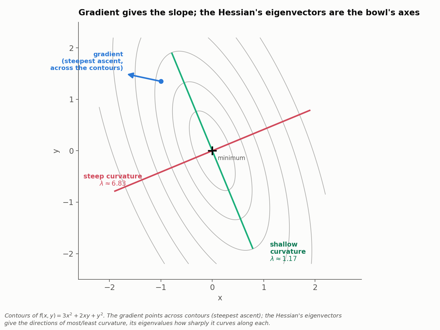
The figure shows both objects on one quadratic bowl. The gradient (blue) points across the contours: purely a slope. The Hessian shows up as the geometry of the bowl itself: its eigenvectors are the axes of the elliptical contours, and its eigenvalues say how sharply the bowl curves along each axis. Along the steep axis (large eigenvalue) the contours crowd together; along the shallow axis (small eigenvalue) they spread apart. The gradient and the Hessian are answering two different questions about the same surface: which way and how curved.
4. Reading the Hessian: eigenvalues and shape
Because $H$ is symmetric, it has real eigenvalues and orthogonal eigenvectors, and the eigen-decomposition is the right lens for reading it. In the eigenvector basis the quadratic form $\tfrac{1}{2}\delta^T H \delta$ decouples into independent one-dimensional parabolas, one per eigenvalue. So the signs of the eigenvalues classify the critical point:
- All eigenvalues positive ($H$ positive definite): every direction curves upward. The point is a local minimum - a bowl.
- All eigenvalues negative ($H$ negative definite): every direction curves downward. A local maximum - a dome.
- Mixed signs ($H$ indefinite): up in some directions, down in others. A saddle.
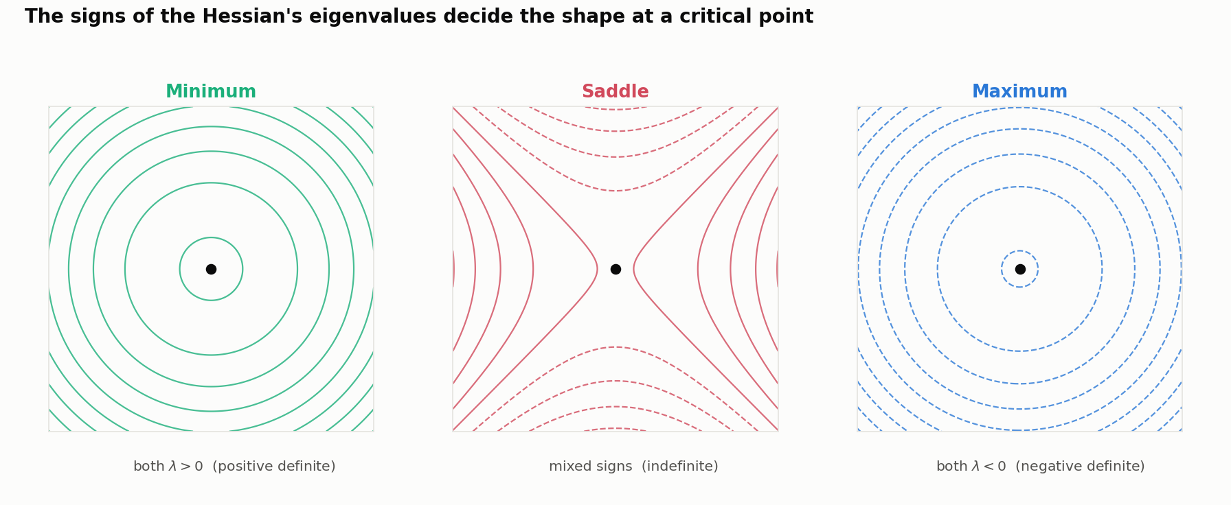
This is not just taxonomy. In high-dimensional deep-learning losses, exact maxima are vanishingly rare; the interesting critical points are saddles, where the gradient is zero but the surface still descends in some directions. Knowing that the Hessian’s mixed signs mark a saddle is what lets an optimizer (or an analysis of one) recognise that it has not actually found a minimum.
Positive-definiteness is also a practical precondition, not just a label. Many algorithms need $H$ (or an approximation of it) to be positive definite so they can be inverted or Cholesky-factorised. When curvature information comes from finite data it can be degenerate - some eigenvalue is zero or slightly negative from noise - and the standard fix is to add a small multiple of the identity, $H + \lambda I$, which lifts every eigenvalue by $\lambda$ and restores definiteness. That is exactly the “damping” term in second-order methods; here it has a clean reading as “nudge the curvature until the bowl is convex again.”
5. Conditioning: why the eigenvalue ratio matters
Eigenvalue signs set the shape; the eigenvalue ratio sets how hard the surface is to optimize. The condition number is
\[\kappa(H) \;=\; \frac{\lambda_{\max}}{\lambda_{\min}}\](for a positive-definite $H$). When $\kappa \approx 1$, the bowl is nearly spherical and gradient descent walks almost straight to the bottom. When $\kappa$ is large, the bowl is a long, narrow ravine - steep across, shallow along - and plain gradient descent zig-zags across the steep walls while crawling along the shallow floor, because a single step size cannot suit both directions at once.
Two everyday consequences follow directly. First, this is why second-order methods help: multiplying the gradient by $H^{-1}$ rescales each eigen-direction by its own curvature, effectively turning the ravine back into a round bowl. Second, it is why feature scaling and normalization matter so much in practice: they reshape the loss so its Hessian is better conditioned, which is the real reason a well-scaled problem trains faster. Curvature is not an abstraction here; it is the difference between a model that converges in a few epochs and one that thrashes.
6. A tiny worked example
Take a two-variable quadratic:
\[f(x, y) = 3x^2 + 2xy + y^2\]Its gradient is
\[\nabla f = \begin{bmatrix} 6x + 2y \\[4pt] 2x + 2y \end{bmatrix}\]and its Jacobian is that gradient transposed, the row vector $\begin{bmatrix} 6x + 2y & 2x + 2y \end{bmatrix}$. (For a scalar function the two carry the same numbers; the shape convention just reflects whether we are thinking “steepest-ascent direction,” a column, or “derivative operator applied to a step,” a row, so that $J\,\delta$ is a scalar.)
Differentiating once more gives the Hessian, a constant matrix because $f$ is exactly quadratic:
\[H = \begin{bmatrix} 6 & 2 \\[4pt] 2 & 2 \end{bmatrix}\]Now stand at $(x, y) = (1, 1)$. The gradient is $(8, 4)$ - steeper in $x$ than $y$. Take a small step $\delta = (0.1, 0)$, a nudge purely in $x$. The resulting change in the gradient is
\[H \delta = \begin{bmatrix} 6 & 2 \\ 2 & 2 \end{bmatrix}\begin{bmatrix} 0.1 \\ 0 \end{bmatrix} = \begin{bmatrix} 0.6 \\ 0.2 \end{bmatrix}\]Moving in $x$ by $0.1$ changed the $x$-slope by $0.6$ (the diagonal, $H_{11}$) and the $y$-slope by $0.2$ (the off-diagonal, $H_{21}$). That non-zero cross-term is the coupling: nudging one coordinate bends the landscape along the other. Its eigenvalues are $\lambda \approx 6.83$ and $1.17$ (the same numbers labelled on the figure in Section 3), so this bowl is mildly ill-conditioned, $\kappa \approx 5.8$, and tilted off-axis because of that off-diagonal $2$.
7. The least-squares bridge: when the Hessian is built from a Jacobian
The deepest connection between the two objects shows up in least-squares problems, which covers a huge share of ML objectives (regression, reconstruction losses, and more). Suppose we minimise a sum of squared residuals
\[f(x) = \tfrac{1}{2}\, \lVert r(x) \rVert^2, \qquad r : \mathbb{R}^n \to \mathbb{R}^m\]Let $J$ be the Jacobian of the residual $r$. Differentiating carefully gives a gradient and a Hessian:
\[\nabla f = J^T r, \qquad H = J^T J + \sum_{i} r_i \, \nabla^2 r_i\]The Hessian has two pieces: a “nice” part $J^T J$ built purely from first derivatives, and a “curvature-of-the-residual” part weighted by the residuals themselves. The Gauss-Newton approximation drops the second term (it is small when the residuals are small or nearly linear), leaving
\[H \;\approx\; J^T J\]a Hessian assembled entirely out of the Jacobian. This is the precise sense in which “second-order” information can be recovered from “first-order” building blocks, and it is why Gauss-Newton and its cousins are so effective on least-squares losses.
When the residual is exactly linear in the parameters, the dropped term is not just small, it is exactly zero (a linear function has no second derivative), so $H = J^T J$ holds exactly. That is the situation inside a linear layer. For the layer-reconstruction objective that GPTQ minimises,
\[L(\delta W) = \lVert \delta W\, X \rVert_F^2,\]each row’s residual is linear in that row’s weights with Jacobian $X^T$, so the Hessian is the constant matrix
\[H = 2\, X X^T,\]no approximation involved. This is why the GPTQ Hessian is just an outer product of the calibration activations: for a linear layer, the Gauss-Newton identity is exact, and the “Jacobian” of the reconstruction is simply the input matrix $X$. The GPTQ article puts this to work.
8. Where these show up
The Jacobian and the Hessian are the recurring machinery behind a lot of ML, not one-off tools:
- Backpropagation is the chain rule applied to Jacobians: each layer contributes a Jacobian, and reverse-mode autodiff multiplies them right-to-left to get the gradient efficiently.
- Newton’s method takes the step $x_{t+1} = x_t - H^{-1}\nabla f$, using curvature to rescale the gradient. It converges far faster than gradient descent near a minimum, but forming and inverting an $n \times n$ Hessian is impractical at scale, which is why quasi-Newton methods (L-BFGS) approximate $H^{-1}$ cheaply from a history of gradients.
- Fisher information, central to natural-gradient methods and to the theory of maximum likelihood, is a Hessian of the (expected) log-likelihood.
- Second-order model compression - Optimal Brain Surgeon, Optimal Brain Quantization, and GPTQ - all derive their pruning or quantization updates from a second-order expansion of a loss around trained weights, using the (inverse) Hessian to decide how to compensate for each change.
Wrap-up
The gradient answers which way; the Hessian answers how curved. The Jacobian is the general first-derivative object that specializes to the gradient for a scalar function, and, through the Gauss-Newton identity, it is also the raw material the Hessian is built from on least-squares problems. Read the Hessian through its eigenvalues - signs for shape (minimum, maximum, saddle), the ratio for conditioning - and most second-order methods stop looking like magic: they are all just exploiting curvature where the slope alone runs out of information. When a “Hessian” turns up in an algorithm, this is the picture to bring back to it.