Connection between KL Divergence & Cross Entropy

What’s the connection between KL Divergence and Cross Entropy?

The previous article used KL to compare two aggregate distributions - a training profile against live traffic - for drift monitoring. Here the same quantity does a different job, one example at a time: $P$ is the target distribution for a single label and $Q$ is the classifier’s predicted distribution, and cross-entropy is the loss that pulls one toward the other. This connects the definitions of information theory directly to the loss function that trains almost every probabilistic classifier. Let’s build it up with a coin-toss experiment.

The Connection: KL Divergence and Cross-Entropy

The key relationship is an exact identity:

\[\text{Cross-Entropy}(P, Q) = \text{KL Divergence}(P \Vert Q) + \text{Entropy}(P)\]

Where:

• $P$ (target distribution): the distribution of the True Coin, the ground truth we are trying to match. (We rarely observe $P$ in full - more on that below - but for a coin we can reason about it directly.)
• $Q$ (model distribution): the Simulating Coin, our model’s prediction.
• $\text{Entropy}(P)$: the inherent uncertainty of the True Coin. Crucially it depends only on $P$, not on our model $Q$, so with $P$ fixed it is a constant as far as training is concerned.

That last point is the whole trick, but it needs stating precisely. Because the two objectives differ by an additive constant in $Q$ (not a proportional factor), they have the same minimizer:

\[\underbrace{H(P, Q)}_{\text{what we minimize}} = \underbrace{H(P)}_{\text{constant in } Q} + D_{\text{KL}}(P \Vert Q).\]

Minimizing $H(P,Q)$ over the model’s parameters therefore minimizes $D_{\text{KL}}(P \Vert Q)$ exactly: shifting the whole curve down by $H(P)$ changes its height, never the location of its minimum. (Writing “$\propto$” is a common shorthand, but this is not proportionality; it is equality up to an additive constant.) This is the core reason cross-entropy is the loss for probabilistic classifiers: driving it down drives the model’s predicted distribution toward the target, as close as the data, model capacity, and optimization allow.

Step-by-Step Derivation (The Coin Flip Example)

Let’s define our coin flip scenario (a Bernoulli trial).

• Heads ($H$): Outcome is 1.
• Tails ($T$): Outcome is 0.

Definitions

1. True Coin ($P$): The true, observed distribution (the ground truth, which we observe in our training data).
   • $P(H) = p$ (The true probability of heads)
   • $P(T) = 1 - p$
2. Simulating Coin ($Q$): Our model’s predicted distribution (the output of our neural network).
   • $Q(H) = q$ (The model’s predicted probability of heads)
   • $Q(T) = 1 - q$

A. Deriving KL Divergence

KL Divergence measures the dissimilarity between $P$ and $Q$.

\[KL(P || Q) = \sum_{i \in \{H, T\}} P(i) \cdot \log\left(\frac{P(i)}{Q(i)}\right)\] \[KL(P || Q) = P(H) \log\left(\frac{P(H)}{Q(H)}\right) + P(T) \log\left(\frac{P(T)}{Q(T)}\right)\]

Substitute the probabilities ($p$ and $q$):

\[KL(P || Q) = p \log\left(\frac{p}{q}\right) + (1-p) \log\left(\frac{1-p}{1-q}\right)\]

Using the log rule $\log(a/b) = \log(a) - \log(b)$:

\[KL(P || Q) = p [\log(p) - \log(q)] + (1-p) [\log(1-p) - \log(1-q)]\]

Rearrange the terms:

\[KL(P || Q) = \underbrace{\left[ -p \log(q) - (1-p) \log(1-q) \right]}_{\text{Term 1}} + \underbrace{\left[ p \log(p) + (1-p) \log(1-p) \right]}_{\text{Term 2}}\]

B. Deriving Cross-Entropy and Entropy

1. Cross-Entropy ($H(P, Q)$):

Cross-Entropy measures the average number of bits needed to encode events from the true distribution $P$ when using the simulating distribution $Q$:

\[H(P, Q) = \sum_{i \in \{H, T\}} -P(i) \log(Q(i))\] \[H(P, Q) = -P(H) \log(Q(H)) - P(T) \log(Q(T))\]

Substitute the probabilities:

\[H(P, Q) = -p \log(q) - (1-p) \log(1-q)\]

Notice this is exactly Term 1 from the KL derivation.

2. Entropy ($H(P)$):

Entropy measures the average number of bits needed to encode events from the true distribution $P$ using the true distribution $P$:

\[H(P) = \sum_{i \in \{H, T\}} -P(i) \log(P(i))\] \[H(P) = -p \log(p) - (1-p) \log(1-p)\]

If we look back at Term 2 from the KL derivation, Term 2 is simply $-H(P)$.

C. The Final Connection

Substituting the definitions back into the expanded KL formula:

\[KL(P || Q) = \underbrace{\left[ -p \log(q) - (1-p) \log(1-q) \right]}_{\text{Cross-Entropy (H(P, Q))}} - \underbrace{\left[ -p \log(p) - (1-p) \log(1-p) \right]}_{\text{Entropy (H(P))}}\]

Therefore:

\[KL(P || Q) = H(P, Q) - H(P)\]

Rearranging this gives us the fundamental relationship:

\[H(P, Q) = KL(P || Q) + H(P)\]

Since $H(P)$ (the true coin’s inherent uncertainty) is fixed by the data, minimizing the Cross-Entropy $H(P, Q)$ achieves the goal of minimizing the dissimilarity: $KL(P \Vert Q)$.

Seeing the Identity: A Numerical Coin Example

The algebra is clearer with numbers. Fix the true coin at $p = 0.8$, so its entropy floor is $H(P) = -0.8\ln 0.8 - 0.2\ln 0.2 \approx 0.500$ nats. Now sweep the model’s prediction $q$ and watch the cross-entropy $H(P,Q) = -0.8\ln q - 0.2\ln(1-q)$:

Model $q$	Cross-entropy $H(P,Q)$	KL above the floor	Interpretation
0.8	0.500	0.000	model matches the truth (the minimum)
0.6	0.592	0.092	under-confident
0.95	0.640	0.140	over-confident
0.5	0.693	0.193	no better than a fair-coin guess
0.05	2.407	1.906	confidently wrong (huge penalty)

Plotted against $q$, cross-entropy is a bowl whose bottom sits exactly on the entropy floor $H(P)$, reached only when $q = p$. Everywhere else, the height above the floor is precisely the KL divergence:

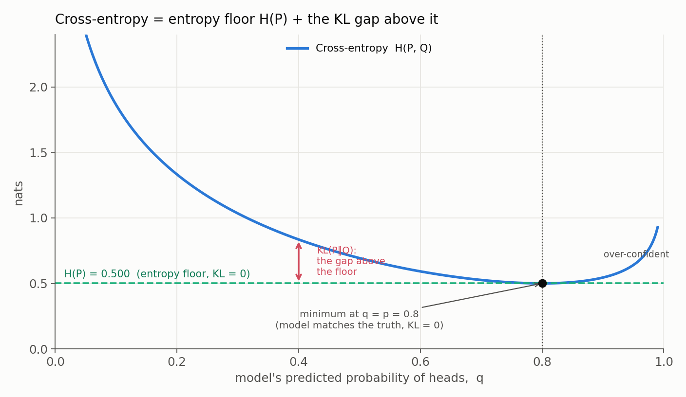
Two things the picture makes obvious. The minimum is at $q = p$, not at $q = 1$: cross-entropy rewards honest probabilities, not maximally confident ones. And the left wall is brutal - a confident wrong prediction ($q \to 0$ when the truth leans heads) sends the loss toward infinity. That is the support condition worth stating outright: if $P(i) > 0$ but $Q(i) = 0$, both cross-entropy and forward KL are infinite. It is exactly why a confidently wrong model is punished so hard. (A note on units: natural logs give nats, base-2 logs give bits; the base rescales the loss but never moves its minimum.)

From a Single Label to a Loss: Cross-Entropy as Log-Likelihood

Here is the step the coin story skips, and the one that matters most in practice. In a real problem we do not observe the true distribution $P(Y \mid X)$. We observe three separate things:

• the population: the true conditional $P(Y \mid X)$, which is unknown;
• the model: the predicted distribution $Q_\theta(Y \mid X)$ with parameters $\theta$;
• the training data: a finite set of examples $(x_i, y_i)$.

So where does a “target distribution $P$” come from for a single training example whose label is just, say, “cat”? We use the one-hot empirical distribution for that example: all the mass on the observed class. For a one-hot target, $H(P) = 0$, the entropy floor vanishes, and per-example cross-entropy equals the KL divergence - both collapsing to a single term, $-\log Q_\theta(y_i \mid x_i)$.

Averaging over the dataset gives the training objective:

\[\widehat{L}(\theta) = -\frac{1}{n}\sum_{i=1}^{n} \log Q_\theta(y_i \mid x_i).\]

This is precisely the negative average log-likelihood of the data under the model. Minimizing empirical cross-entropy is maximum-likelihood estimation of the conditional model. And across the population, minimizing the expected cross-entropy targets the true conditional:

\[\mathbb{E}_X\,H\big(P(\cdot\mid X),\, Q_\theta(\cdot\mid X)\big) = \mathbb{E}_X\,H\big(P(\cdot\mid X)\big) + \mathbb{E}_X\,D_{\text{KL}}\big(P(\cdot\mid X)\,\Vert\,Q_\theta(\cdot\mid X)\big),\]

where the entropy term varies with $x$ but its expectation is still constant in $\theta$. The one-hot label is our finite-sample stand-in for that unknown conditional; with enough data, driving the empirical loss down chases the real thing - subject, always, to model capacity, regularization, optimization, and any train/deploy distribution mismatch.

The Forms We Actually Use

Binary cross-entropy. For a label $y \in \{0, 1\}$ and predicted probability $q$ of the positive class:

\[\ell(y, q) = -y\log q - (1-y)\log(1-q).\]

The one-hot label collapses this to a single term: if $y = 1$ the loss is $-\log q$; if $y = 0$ it is $-\log(1-q)$. (This is exactly the coin formula, with the label playing the role of a $p \in \{0, 1\}$.)

Multiclass cross-entropy. For a one-hot target $\mathbf{y}$ over $K$ classes and predicted class probabilities $\mathbf{q}$ (typically from a softmax):

\[\ell(\mathbf{y}, \mathbf{q}) = -\sum_{k=1}^{K} y_k \log q_k = -\log q_{\text{true class}}.\]

Only the predicted probability of the correct class enters the loss - the direct link between cross-entropy and softmax classifiers.

Soft labels. Sometimes the target is deliberately not one-hot: label smoothing spreads a little mass onto the other classes, and knowledge distillation trains against a teacher’s full probability vector. The same cross-entropy formula applies, but now $H(P) \neq 0$, so the minimum achievable loss is the (nonzero) entropy of the soft target rather than zero.

A Note on Implementation: Feed Logits, Not Probabilities

One practical trap. Production libraries almost always want the model’s raw logits (pre-softmax scores), not already-normalized probabilities, so they can fuse the log-softmax and the negative-log-likelihood into one numerically stable step (via the log-sum-exp trick). PyTorch’s CrossEntropyLoss, for example, expects unnormalized logits. A few rules follow:

• use CrossEntropyLoss for mutually exclusive multiclass problems (logits in), and BCEWithLogitsLoss for binary or multi-label logits;
• do not apply softmax (or sigmoid) and then the with-logits loss - that double-counts the normalization;
• avoid hand-rolling log(softmax(x)); the fused versions are what keep gradients stable when a logit is large.

What Cross-Entropy Does Not Guarantee

Cross-entropy optimizes probability quality, which is not the same as every property we might care about. A low log loss does not by itself guarantee low error at a chosen threshold, calibration on shifted deployment data, fairness across subgroups, causal validity, or robustness to out-of-distribution inputs. It is one axis among several, and it helps to know what each metric actually rewards:

Metric	Rewards	Mainly sensitive to
Cross-entropy / log loss	accurate, calibrated probabilities	confident mistakes
Accuracy	correct hard labels	the chosen threshold / argmax
ROC-AUC	ranking positives above negatives	pairwise order only
Brier score	squared probability error	calibration and refinement

Cross-entropy and ranking metrics answer different questions: a model can post an excellent ROC-AUC yet output poorly calibrated probabilities - the “ranking is not calibration” point from the metrics article. Train with cross-entropy for good probabilities; evaluate with whichever metric matches the decision at hand.

Summary

• The identity: $H(P, Q) = H(P) + D_{\text{KL}}(P \Vert Q)$. With $P$ fixed, $H(P)$ is constant in the model, so minimizing cross-entropy minimizes KL - they share a minimizer because they differ by an additive constant, not a proportional one.
• The bridge: with one-hot targets, per-example cross-entropy is $-\log Q_\theta(y_i \mid x_i)$, so minimizing average cross-entropy is maximum-likelihood estimation of the conditional model.
• The caveats: the true $P(Y\mid X)$ is never observed (one-hot labels are its finite-sample stand-in); confidently wrong predictions cost infinitely; feed logits to the loss; and a low log loss speaks to probability quality, not to accuracy, calibration under shift, or fairness.