Support Vector Machines, Part 2: The Dual and Support Vectors
Derive the SVM dual with Lagrange multipliers, see why the dual is often preferred over the primal, and read off the support vectors through the KKT conditions.
- Geometry, margins, and hinge loss
- The dual and support vectors You are here
- The kernel trick
- One-Class SVM
Part 1 built the linear SVM: the margin, the hard-margin primal, and the soft-margin hinge-loss objective. This part re-expresses that problem in its dual form. We derive the dual with the Lagrangian, see when it is preferable to the primal, and read off the support vectors through the KKT conditions. Part 3 then uses one property of this dual, its dependence on dot products, to unlock non-linear boundaries.
1. From Primal to Dual: The Lagrangian
Deriving the Dual Function
Solving the primal problem directly can be complex. We can re-frame it into a more manageable form called the Dual Problem using the technique of Lagrange Multipliers.
Form the Lagrangian: We introduce non-negative Lagrange multipliers $\alpha_i \ge 0$ (one for each constraint) and form the Lagrangian function, $\mathcal{L}$:
\[\mathcal{L}(\mathbf{w}, b, \mathbf{\alpha}) = \underbrace{\frac{1}{2}\|\mathbf{w}\|^2}_{\text{Original Objective}} + \underbrace{\sum_{i=1}^{n} \alpha_i [1 - y_i(\mathbf{w} \cdot \mathbf{x}_i + b)]}_{\text{Constraints with Multipliers }\alpha_i \ge 0}\]Let’s expand the terms inside the sum to make differentiation easier:
\[\mathcal{L}(\mathbf{w}, b, \alpha) = \frac{1}{2}(\mathbf{w} \cdot \mathbf{w}) - \sum_{i=1}^{n} \alpha_i y_i (\mathbf{w} \cdot \mathbf{x}_i) - \sum_{i=1}^{n} \alpha_i y_i b + \sum_{i=1}^{n} \alpha_i\]To find the Dual Function $W(\alpha)$, we must minimize $\mathcal{L}$ with respect to the primal variables $\mathbf{w}$ and $b$. We do this by calculating gradients and setting them to zero.
Step 1: Derivative with respect to w
We take the partial derivative of $\mathcal{L}$ with respect to the vector $\mathbf{w}$:
\[\frac{\partial \mathcal{L}}{\partial \mathbf{w}} = \frac{\partial}{\partial \mathbf{w}}\left(\frac{1}{2}\mathbf{w} \cdot \mathbf{w}\right) - \frac{\partial}{\partial \mathbf{w}}\left(\sum_{i=1}^{n} \alpha_i y_i (\mathbf{w} \cdot \mathbf{x}_i)\right) - 0 + 0\] \[\nabla_\mathbf{w} \mathcal{L} = \mathbf{w} - \sum_{i=1}^{n} \alpha_i y_i \mathbf{x}_i\]Setting this to zero gives us our first crucial relationship:
\[\mathbf{w} = \sum_{i=1}^{n} \alpha_i y_i \mathbf{x}_i \quad \text{--- (Equation 1)}\]Step 2: Derivative with respect to b
Now, we take the derivative with respect to the bias $b$:
\[\frac{\partial \mathcal{L}}{\partial b} = 0 - 0 - \frac{\partial}{\partial b}\left(b \sum_{i=1}^{n} \alpha_i y_i\right) + 0\] \[\frac{\partial \mathcal{L}}{\partial b} = - \sum_{i=1}^{n} \alpha_i y_i\]Setting this to zero gives us our second constraint:
\[\sum_{i=1}^{n} \alpha_i y_i = 0 \quad \text{--- (Equation 2)}\]Step 3: Substitute Back to Find W(α)
Now, we substitute (Equation 1) and (Equation 2) back into the original Lagrangian to eliminate $\mathbf{w}$ and $b$.
\[\mathcal{L} = \frac{1}{2}\underbrace{(\mathbf{w} \cdot \mathbf{w})}_{\text{Sub Eq. 1}} - \sum_{i=1}^{n} \alpha_i y_i \mathbf{x}_i \cdot \underbrace{\mathbf{w}}_{\text{Sub Eq. 1}} - b \underbrace{\sum_{i=1}^{n} \alpha_i y_i}_{\text{Eq. 2 says this is 0}} + \sum_{i=1}^{n} \alpha_i\]A. Expand the first term:
\[\frac{1}{2}(\mathbf{w} \cdot \mathbf{w}) = \frac{1}{2} \left( \sum_{i=1}^n \alpha_i y_i \mathbf{x}_i \right) \cdot \left( \sum_{j=1}^n \alpha_j y_j \mathbf{x}_j \right) = \frac{1}{2} \sum_{i=1}^n \sum_{j=1}^n \alpha_i \alpha_j y_i y_j (\mathbf{x}_i \cdot \mathbf{x}_j)\]B. Expand the second term:
\[- \sum_{i=1}^n \alpha_i y_i \mathbf{x}_i \cdot \mathbf{w} = - \sum_{i=1}^n \alpha_i y_i \mathbf{x}_i \cdot \left( \sum_{j=1}^n \alpha_j y_j \mathbf{x}_j \right) = - \sum_{i=1}^n \sum_{j=1}^n \alpha_i \alpha_j y_i y_j (\mathbf{x}_i \cdot \mathbf{x}_j)\]C. Combine Everything: Notice that Term B is exactly $-2$ times Term A.
\[\mathcal{L} = \left[ \frac{1}{2} \sum \sum \dots \right] - \left[ \sum \sum \dots \right] - 0 + \sum_{i=1}^n \alpha_i\]Simplifying $(\frac{1}{2} X - X = -\frac{1}{2} X)$ gives the final Dual Objective Function:
\[W(\alpha) = \sum_{i=1}^{n} \alpha_i - \frac{1}{2} \sum_{i=1}^{n} \sum_{j=1}^{n} \alpha_i \alpha_j y_i y_j (\mathbf{x}_i \cdot \mathbf{x}_j)\]Bridge: The Two-Step Process to Find the Saddle Point
Think of solving the Lagrangian as a strategic game between two opposing players.
- Player 1 (Primal Player): Controls
wandb. Their goal is to minimizeL. - Player 2 (Dual Player): Controls
α. Their goal is to maximizeL.
A stable solution, or equilibrium, is found at a saddle point: a point that is a minimum in the primal direction (w, b) and a maximum in the dual direction (α). We find this point in two steps:
Step 1: Minimize with Respect to w and b (This defines W(α))
First, we let the dual player fix a set of multipliers, α. Now, the primal player gets to make their move. They take this fixed α and find the values of w and b that make L as small as possible.
This step is exactly the minimization we performed above: we minimize L(w, b, α) over w and b.
When we do this (by taking partial derivatives and setting them to zero), we get expressions for w and b that depend only on α. The result of this minimization is a new function, which we call the Lagrange dual function, W(α).
The inf (infimum, or minimum) here explicitly shows that W(α) is defined as the result of the minimization of L with respect to the primal variables.
Step 2: Maximize the Result with Respect to α
Now it’s the dual player’s turn. They know that for any α they choose, the primal player will minimize L to get the value W(α). The dual player’s goal is to choose an α that makes this resulting value as large as possible.
Therefore, the second step is to maximize W(α).
Why maximize? Because the dual function W(α) provides a lower bound on the true optimal value of our original problem. To get the best, tightest possible lower bound, we must find the highest point of this floor, which means maximizing it.
An Analogy: The King in the Mountain Pass
Imagine a king who wants to find the highest possible camping spot, but he is constrained to only travel along the bottom of mountain valleys. The mountain range represents the function L.
- The east-west direction represents the primal variables (
w,b). - The north-south direction represents the dual variables (
α).
Minimizing L: For any fixed north-south path (
α), the king walks east-west to find the absolute lowest point in that valley. He is minimizing his altitude for that path. This gives him one point,W(α).Maximizing W(α): The king repeats this for every possible north-south path. He now has a collection of the lowest points from all the valleys. To find the best possible camping spot under his constraint, he chooses the highest among all these low points. He is maximizing the function
W(α).
The final spot is a saddle point: it’s the lowest point in the east-west direction, but the highest point when viewed along the north-south collection of valley floors.
The Guarantee: Strong Duality
For the SVM, a property called strong duality holds, guaranteeing that the minimum of the primal problem is exactly equal to the maximum of the dual problem. This is worth stating precisely, because convexity alone is not enough: a convex problem guarantees only weak duality (the dual is a lower bound). Equality also requires a constraint qualification. The SVM primal is a convex quadratic program, and when the data are separable a strictly feasible point exists after rescaling, so Slater’s condition is satisfied. Convex QP plus Slater is what delivers strong duality here (the soft-margin formulation with slack variables is strictly feasible under the standard setup as well).
\[\min (\text{Primal Problem}) = \max (\text{Dual Problem})\] \[\min_{\mathbf{w},b} \left( \max_{\alpha \ge 0} \mathcal{L}(\mathbf{w}, b, \mathbf{\alpha}) \right) = \max_{\alpha \ge 0} \left( \min_{\mathbf{w},b} \mathcal{L}(\mathbf{w}, b, \mathbf{\alpha}) \right)\]This is why this two-step process works and why solving the “max of the min” (the dual problem) gives us the answer to our original “min of the max” (the primal problem).
The Logic Chain: Primal to Dual
Here is how we logically move from the original minimization problem to the maximization of the dual we just derived.
1. The Original Primal Problem
Our goal is to find the minimum weights while satisfying constraints:
\[\min_{\mathbf{w}, b} \frac{1}{2}\|\mathbf{w}\|^2 \quad \text{subject to } y_i(\mathbf{w}\cdot\mathbf{x}_i+b) \ge 1\]2. $\min(\max(\text{Lagrangian}))$
We convert the constrained problem into an unconstrained “Min-Max” problem using the Lagrangian.
\[P^* = \min_{\mathbf{w}, b} \left( \max_{\alpha \ge 0} \mathcal{L}(\mathbf{w}, b, \alpha) \right)\]- Logic: The inner maximization acts as a “validity check.”
- If constraints are violated, $\max \mathcal{L} = \infty$.
- If constraints are satisfied, $\max \mathcal{L} = \frac{1}{2}\|\mathbf{w}\|^2$ (since the penalty term becomes 0).
- The outer minimization will naturally avoid the $\infty$ cases and choose the smallest valid weights. Thus, this is equivalent to Step 1.
3. Strong Duality: ($\min(\max(\text{Lagrangian})) \equiv \max(\min(\text{Lagrangian}))$)
This is the critical bridge. Because the SVM optimization problem is convex (a quadratic objective with linear constraints) and satisfies Slater’s condition, Strong Duality holds.
Strong Duality asserts that the order of Min and Max can be swapped without changing the result.
\[\underbrace{\min_{\mathbf{w}, b} \max_{\alpha \ge 0} \mathcal{L}(\mathbf{w}, b, \alpha)}_{\text{Primal Problem } (P^*)} = \underbrace{\max_{\alpha \ge 0} \min_{\mathbf{w}, b} \mathcal{L}(\mathbf{w}, b, \alpha)}_{\text{Dual Problem } (D^*)}\]- Without Strong Duality (Weak Duality), the Dual is only a lower bound ($D^\ast \le P^\ast$).
- With Strong Duality, they are equal ($D^\ast = P^\ast$).
4. $\max(\min(\text{Lagrangian})) \Rightarrow \max(\text{Dual})$
Now we solve the right side of the equation from Step 3.
- Inner Minimization: We perform $\min_{\mathbf{w}, b} \mathcal{L}$. This is exactly what we did in the derivation above (taking derivatives w.r.t
wandb). The result of this calculation is the function $W(\alpha)$. - Outer Maximization: We are left with the final step:
This is why we end up maximizing the dual formulation to solve the original minimization problem.
Recovering the Classifier and Making Predictions
Solving the dual gives us the multipliers $\alpha$, but a usable classifier needs $\mathbf{w}$ and $b$. Collecting the full dual problem in one place, with every constraint beside the objective (hard-margin form):
\[\begin{aligned} & \max_{\alpha} & & \sum_{i=1}^{n} \alpha_i - \frac{1}{2} \sum_{i=1}^{n} \sum_{j=1}^{n} \alpha_i \alpha_j y_i y_j (\mathbf{x}_i \cdot \mathbf{x}_j) \\ & \text{subject to} & & \alpha_i \ge 0 \quad \text{and} \quad \sum_{i=1}^{n} \alpha_i y_i = 0. \end{aligned}\]For the soft-margin C-SVM (introduced in Part 1), the only change is an upper bound on each multiplier: $0 \le \alpha_i \le C$. From the optimal $\alpha$ we recover the model in three steps:
Weights. Equation 1 gives $\mathbf{w} = \sum_i \alpha_i y_i \mathbf{x}_i$. Only support vectors (nonzero $\alpha_i$) contribute.
Bias. Pick any support vector $\mathbf{x}_k$ that sits exactly on the margin. It satisfies $y_k(\mathbf{w} \cdot \mathbf{x}_k + b) = 1$, so $b = y_k - \mathbf{w} \cdot \mathbf{x}_k$ (using $y_k = 1/y_k$ for labels $\pm 1$). In the soft-margin case, prefer the free support vectors with $0 < \alpha_k < C$ (the ones genuinely on the margin) and average the estimate across all of them for numerical stability.
Prediction. Classify a new point by the sign of the decision score, $\hat y = \text{sign}(\mathbf{w} \cdot \mathbf{x} + b)$.
Without this recovery step the derivation stops one line short of a working model.
The Worked Example, Now Through the Dual
Recall the eight-point dataset from Part 1: class $+1$ at (2,2), (2,3), (3,2), (3,3) and class $-1$ at (0,0), (0,1), (1,0), (1,1). Solving the dual assigns $\alpha = 1$ to the two support vectors (2,2) and (1,1) and $\alpha = 0$ to everyone else, which we can check against the two dual constraints and then use to rebuild the model:
- Equality constraint: $\sum_i \alpha_i y_i = (1)(+1) + (1)(-1) = 0$. ✓
- Weights: $\mathbf{w} = \sum_i \alpha_i y_i \mathbf{x}_i = (+1)(2,2) + (-1)(1,1) = (1,1)$.
- Bias from the margin support vector (2,2): $b = y_k - \mathbf{w}\cdot\mathbf{x}_k = 1 - (1,1)\cdot(2,2) = 1 - 4 = -3$.
This reproduces the $\mathbf{w} = (1,1)$, $b = -3$ we found geometrically in Part 1, now assembled entirely from the dual multipliers. The dual_coef_ array printed by the scikit-learn snippet in Part 1 was exactly $\alpha_i y_i = [-1, +1]$ for the two support vectors.
2. Primal versus Dual: Which to Solve
That’s an excellent question that gets to the practical reasons behind the mathematical formulation of Support Vector Machines.
It’s not that solving the primal problem is always inherently “harder” in a theoretical sense, but the dual problem is often computationally more efficient and flexible, especially in the scenarios where SVMs truly shine.
Here’s a breakdown of the key reasons why the dual problem is often preferred over the primal:
1. The “Tall vs. Wide Data” Dilemma (Features vs. Data Points)
Let’s say we have a dataset with:
- n = number of data points (samples)
- d = number of features (dimensions)
Primal Problem:
The primary variable we are solving for in the primal problem is the weight vector w, which has a size equal to the number of features, d.
- When
dis very large (thousands of features in text or image analysis), solving directly for a massivewvector is the natural bottleneck.
Dual Problem:
The primary variables we are solving for in the dual problem are the Lagrange multipliers α, one for each data point. So we are solving for n variables.
- When
n(the number of samples) is smaller thand, solving fornmultipliers is the more natural size of problem than solving fordweights.
Conclusion: For “wide” datasets with more features than samples ($d > n$), common in bioinformatics and text classification, the dual is the more natural size of problem.
A caution on complexity: the number of primal versus dual variables is useful intuition, but it is not a runtime model. Actual cost depends on the solver, the loss, sparsity, the kernel, the stopping tolerance, cache behavior, and data geometry, so avoid quoting a single big-O for “the SVM.” For concrete numbers, name the implementation: scikit-learn notes that its libsvm-based kernel training scales between roughly $O(n_\text{features} \cdot n_\text{samples}^2)$ and $O(n_\text{features} \cdot n_\text{samples}^3)$ depending on data and cache, while its specialized linear solver (LinearSVC) scales far better on large linear problems. A few practical rules of thumb:
- A nonlinear kernel commits us to the dual and to storing or caching a Gram matrix, which grows poorly with the number of samples.
- For a large linear problem,
LinearSVCor stochastic solvers (SGDClassifier) are usually far more scalable than a kernelSVC.
2. The Power of the Kernel Trick
This is arguably the most important reason for using the dual formulation.
Primal Problem:
The primal problem is expressed in terms of the weight vector w. To classify a new point x, we calculate w ⋅ x + b. This formulation requires us to know the coordinates of our data in the feature space. If we want to use a non-linear model, we would have to first explicitly map our data into a higher-dimensional space using a transformation function φ(x) and then solve for w in that new, potentially infinite-dimensional space. This is often impractical or outright impossible.
Dual Problem:
The dual problem’s objective function and the final decision function depend on the data only through dot products of the feature vectors ($x_i \cdot x_j$).
Decision Function: $f(\mathbf{x}) = \text{sign} \left( \sum_{i=1}^{n} \alpha_i y_i (\mathbf{x}_i \cdot \mathbf{x}) + b \right)$
This is a crucial property. It means we can use the kernel trick:
- Choose a kernel function K($x_i, x_j$) that calculates the dot product in a higher-dimensional space, without ever having to transform the data. For example, the Radial Basis Function (RBF) kernel implicitly maps data to an infinite-dimensional space.
- Simply replace the dot product ($x_i \cdot x_j$) with the kernel function K($x_i, x_j$) in the dual formulation.
Conclusion: The dual problem provides an elegant and efficient way to train non-linear SVMs on complex datasets where a linear boundary would fail. The primal problem does not naturally accommodate the kernel trick.
3. Simpler Constraints
From a numerical optimization perspective, the nature of the constraints matters.
Primal Problem Constraints: We have n inequality constraints of the form $y_i(\mathbf{w} \cdot \mathbf{x}_i + b) \ge 1$. These are linear inequalities, which can be complex to handle for some optimization algorithms.
Dual Problem Constraints: We have simpler constraints:
- n “box” constraints: $0 \le \alpha_i \le C$ (in the soft-margin case).
- One equality constraint: $\sum \alpha_i y_i = 0$.
For many quadratic programming (QP) solvers, this set of constraints is easier to work with. The structure of the dual problem led to the development of highly efficient algorithms like Sequential Minimal Optimization (SMO), which breaks the large QP problem into a series of the smallest possible QP problems that can be solved analytically.
Summary Table
| Aspect | Primal Problem | Dual Problem | Advantage |
|---|---|---|---|
| Variables to Solve | Weight vector w (size d) | Lagrange multipliers α (size n) | Dual, if #features > #samples |
| Kernel Trick | Not directly applicable | Naturally incorporates kernels by replacing dot products | Dual, enables non-linear models |
| Constraints | n linear inequality constraints | n box constraints + 1 equality constraint | Dual, structure is often easier for QP solvers |
| Ideal Use Case | Linear SVMs where d is much smaller than n. | Non-linear SVMs, or when d > n. |
In modern machine learning libraries, if we are explicitly using a linear kernel with a large number of samples, the implementation might solve the primal problem (e.g., using methods like Stochastic Gradient Descent). However, for the powerful, non-linear capabilities that made SVMs famous, the dual problem is the key.
3. Support Vectors and the KKT Conditions
The answer to both questions lies in a set of conditions from optimization theory called the Karush-Kuhn-Tucker (KKT) conditions. Let’s break them down.
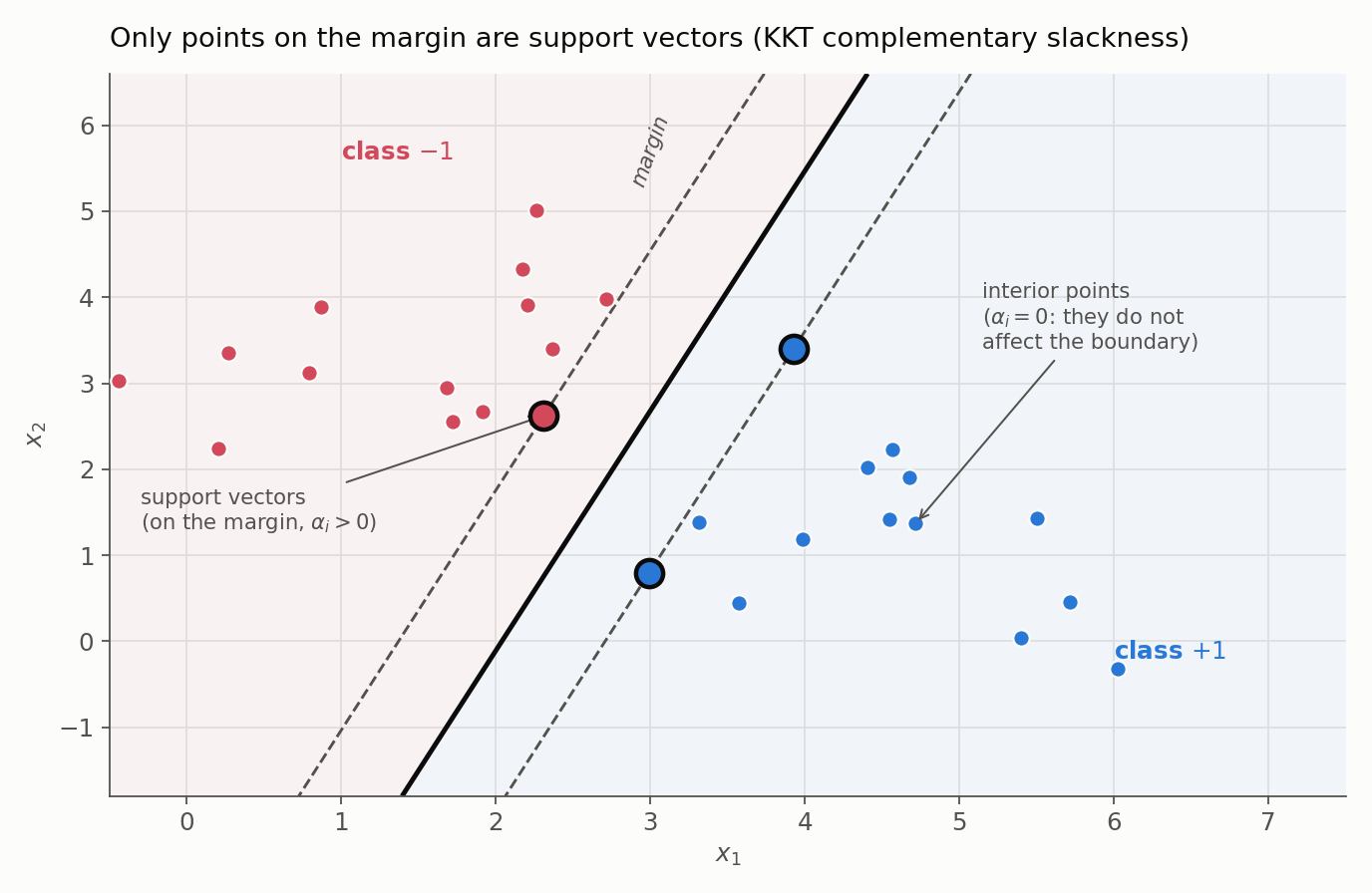
The figure previews where this is heading: of all the training points, only the handful sitting exactly on the margin (circled) end up as support vectors with $\alpha_i > 0$. Every interior point has $\alpha_i = 0$ and could be deleted without moving the boundary. The KKT conditions are what make this precise.
1. How do we determine which points will act as support vectors?
We don’t determine this in advance. The optimization algorithm discovers which points are the support vectors as a result of finding the maximum margin hyperplane.
A point $\mathbf{x}_i$ is defined as a support vector if it lies exactly on one of the margin boundaries. In other words, its “functional margin” is exactly 1.
Mathematically, a point $\mathbf{x}_i$ is a support vector if it satisfies:
\[y_i(\mathbf{w} \cdot \mathbf{x}_i + b) = 1\]Let’s look at the possibilities for any given data point once the optimal hyperplane ($\mathbf{w}, b$) has been found:
Case 1: The point is on the margin. $y_i(\mathbf{w} \cdot \mathbf{x}_i + b) = 1$. These are the support vectors. They are the most critical points because they are the closest to the decision boundary and define its position.
Case 2: The point is correctly classified and is “off the street” (beyond the margin). $y_i(\mathbf{w} \cdot \mathbf{x}_i + b) > 1$. These points are correctly classified with room to spare. They are not support vectors. If we were to remove one of these points, the optimal hyperplane would not change.
Case 3 (in soft-margin SVM): The point is a margin violator. $y_i(\mathbf{w} \cdot \mathbf{x}_i + b) < 1$. This includes points that are on the wrong side of the hyperplane or are inside the margin. These are also considered support vectors because they influence the final position of the hyperplane.
So, the identity of the support vectors is a direct outcome of the optimization process that finds the w and b that maximize the margin.
2. Why do only the support vectors have non-zero α?
This is the most elegant part of the SVM formulation, and it comes directly from one of the KKT conditions known as complementary slackness.
Recall our primal problem’s constraints:
\[y_i(\mathbf{w} \cdot \mathbf{x}_i + b) \ge 1 \quad \text{or, written differently,} \quad y_i(\mathbf{w} \cdot \mathbf{x}_i + b) - 1 \ge 0\]When we created the Lagrangian dual, we introduced a multiplier $\alpha_i$ for each one of these constraints. The complementary slackness condition for SVM states that for the optimal solution, the following must be true for every single data point:
\[\alpha_i \left( y_i(\mathbf{w} \cdot \mathbf{x}_i + b) - 1 \right) = 0\]This simple equation is a powerful “either-or” statement. For this product to be zero, at least one of its factors must be zero. Let’s analyze the two possibilities for any data point i:
Possibility A: The point is NOT a support vector.
- If a point is not a support vector, it lies correctly classified and beyond the margin.
As we saw above, this means its functional margin is greater than 1:
\[y_i(\mathbf{w} \cdot \mathbf{x}_i + b) > 1\]Therefore, the term in the parenthesis of the KKT condition is not zero:
\[\left( y_i(\mathbf{w} \cdot \mathbf{x}_i + b) - 1 \right) > 0\]- For the entire KKT equation to equal zero, the other factor must be zero.
- Conclusion: For any non-support vector, its multiplier $\alpha_i$ must be 0.
Possibility B: The point IS a support vector.
- If a point is a support vector, it lies exactly on the margin.
This means its functional margin is exactly 1:
\[y_i(\mathbf{w} \cdot \mathbf{x}_i + b) = 1\]Therefore, the term in the parenthesis of the KKT condition is zero:
\[\left( y_i(\mathbf{w} \cdot \mathbf{x}_i + b) - 1 \right) = 0\]- Now the parenthesis is zero, so complementary slackness is satisfied for any non-negative $\alpha_i$. It permits a positive multiplier but does not force one.
- Conclusion: A support vector is allowed a positive multiplier, and in the usual (non-degenerate) case it has one. The logic runs cleanly in the other direction: $\alpha_i > 0 \implies$ the constraint is active, so the point lies on the margin. The reverse implication (“on the margin $\implies \alpha_i > 0$”) is what holds in typical cases but is not guaranteed by KKT alone, because degenerate optima can place a point exactly on the margin with $\alpha_i = 0$.
Summary (Hard Margin)
Position of Point i | Value of $(y_i(\mathbf{w} \cdot \mathbf{x}_i + b) - 1)$ | Value of $\alpha_i$ | Support Vector? |
|---|---|---|---|
| Beyond the margin | $> 0$ | $= 0$ | No |
| On the margin | $= 0$ | $\ge 0$ (typically $> 0$) | Yes |
The Soft-Margin Picture
Real classifiers use the soft margin from Part 1, where the box constraint $0 \le \alpha_i \le C$ splits the support vectors into two kinds. The standard non-degenerate cases are:
| Training-point position | Typical $\alpha_i$ | Interpretation |
|---|---|---|
| Correct and outside the margin | $\alpha_i = 0$ | Not a support vector; absent from $\mathbf{w} = \sum \alpha_i y_i \mathbf{x}_i$ |
| Exactly on the margin | $0 < \alpha_i < C$ | Free support vector |
| Inside the margin or misclassified | $\alpha_i = C$ | Bounded support vector (a margin error) |
One naming caveat: libraries typically call any sample with a nonzero dual coefficient a “support vector,” which is the operational definition used above. Geometric descriptions sometimes reserve the term for points exactly on the margin. We use the operational sense.
This is why solving the dual is so powerful. By finding which $\alpha_i$ are non-zero, we simultaneously identify the support vectors and assemble the decision boundary, $\mathbf{w} = \sum \alpha_i y_i \mathbf{x}_i$. The model is built only from the points that truly matter.
The dual exposes the support vectors and, crucially, expresses everything through dot products of the data. That single fact is the doorway to non-linear SVMs. Continue to Part 3: The Kernel Trick.