Support Vector Machines, Part 3: The Kernel Trick

Support Vector Machines series: Part 1: Geometry, Margins, and Hinge Loss · Part 2: The Dual and Support Vectors · Part 3: The Kernel Trick · Part 4: One-Class SVM for Novelty Detection

Part 2 showed that the SVM dual depends on the training data only through dot products $\mathbf{x}_i \cdot \mathbf{x}_j$. That single fact is what makes non-linear SVMs possible. This part develops the kernel trick, works through the polynomial and RBF kernels, and closes with the practical choices, tuning, multiclass, and regression, that turn the theory into a working model.

1. The Kernel Trick

The Kernel Trick is a powerful and elegant concept that gives SVMs much of their versatility. Let’s break it down, first as a general idea, and then apply it directly to SVM.

The Kernel Trick as a General Idea

At its core, the Kernel Trick is a mathematical shortcut that allows us to work in a very high-dimensional feature space without ever having to actually compute the coordinates of our data in that space.

The Problem: Non-Linear Data

Imagine our data is not separable by a simple straight line. A classic example is data arranged in concentric circles, with one class forming the inner circle and the other the outer ring.

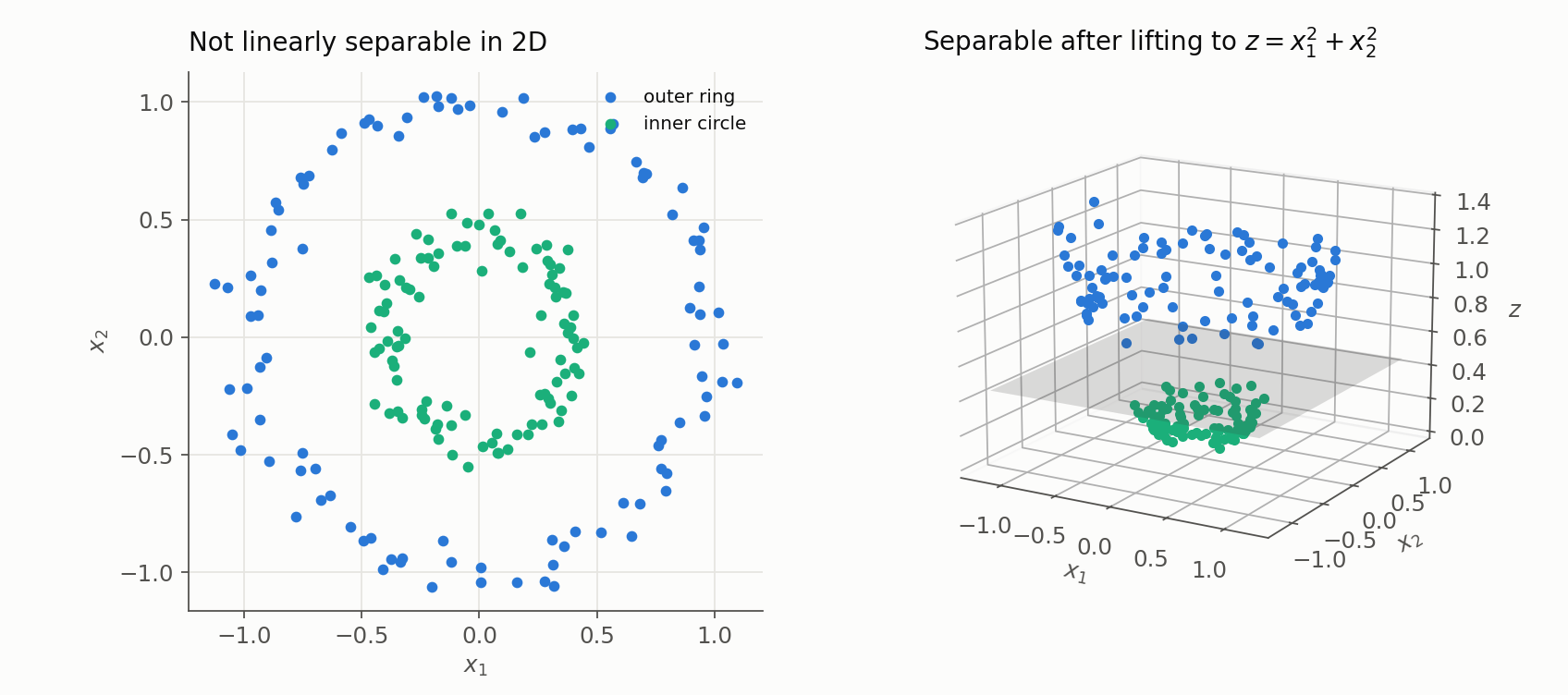
Clearly, no single straight line can separate the inner circle from the outer ring, so a plain linear SVM fails on this data as it stands. The right panel above previews the escape route, the explicit feature map we develop next.

The “Hard Way” Solution: Explicit Feature Mapping

The standard way to solve this is to create new features from the existing ones, hoping that in this new, higher-dimensional feature space, the data becomes linearly separable. This is called feature mapping.

Let’s say a data point is defined by two features, $\mathbf{x} = [x_1, x_2]$. We could define a mapping function, $\phi$, that transforms our 2D data into 3D. A good one for this problem would be to add a third feature that represents the squared distance from the origin:

\[\phi(\mathbf{x}) = \phi([x_1, x_2]) = [x_1, x_2, x_1^2 + x_2^2]\]

This is exactly the lift shown in the right panel above. Applying the transformation, the inner-circle points get a low value for the new third feature $x_1^2 + x_2^2$, while the outer-ring points get a high value, so in this 3D space the data can be separated by a simple flat plane.

The Problems with the “Hard Way”:

1. Computational Cost: Imagine our mapping function $\phi$ transforms the data into a million-dimensional space (or even an infinite-dimensional space!). Calculating the new coordinates for every single data point would be incredibly slow or literally impossible.
2. Finding the Right Map: How do we even know which mapping function $\phi$ will work? Designing good features is a difficult task in itself.

The “Magic” of the Kernel Trick

Here’s the key insight: What if an algorithm doesn’t need the actual coordinates of the points in the high-dimensional space, but only the dot products between them?

Many machine learning algorithms (including SVM) have this property. Their mathematics only require the value of $\phi(\mathbf{x}_i) \cdot \phi(\mathbf{x}_j)$.

A Kernel is a function $K(\mathbf{x}_i, \mathbf{x}_j)$ that gives us the result of this high-dimensional dot product directly from the original low-dimensional vectors, completely bypassing the need to compute the transformation $\phi$.

\[K(\mathbf{x}_i, \mathbf{x}_j) = \phi(\mathbf{x}_i) \cdot \phi(\mathbf{x}_j)\]

Not every similarity function qualifies. For $K$ to correspond to an inner product in some feature space, it must be a valid (Mercer) kernel: on any finite set of points the resulting Gram matrix $K_{ij}$ must be symmetric positive semidefinite. This condition is also what keeps the SVM’s dual objective convex. The polynomial and RBF kernels below both satisfy it.

The Kernel Trick is the act of replacing the expensive, two-step process:

1. Compute $\mathbf{z}_i = \phi(\mathbf{x}_i)$ and $\mathbf{z}_j = \phi(\mathbf{x}_j)$ for all points.
2. Compute the dot product $\mathbf{z}_i \cdot \mathbf{z}_j$.

with a single, cheap step:

1. Compute $K(\mathbf{x}_i, \mathbf{x}_j)$.

This allows us to get all the benefits of working in a high-dimensional space (finding non-linear patterns) with the computational cost of working in the original low-dimensional space.

Applying the Kernel Trick to SVM

Now, let’s see why SVM is the perfect candidate for this trick.

The Opportunity in the Dual Formulation

Recall the dual formulation for the hard-margin SVM, derived in Part 2. The goal is to find the alphas ($\alpha_i$) that maximize:

\[W(\alpha) = \sum_{i=1}^{n} \alpha_i - \frac{1}{2} \sum_{i=1}^{n} \sum_{j=1}^{n} \alpha_i \alpha_j y_i y_j (\mathbf{x}_i \cdot \mathbf{x}_j)\]

Look closely at this equation. The data points $\mathbf{x}_i$ and $\mathbf{x}_j$ are only ever used inside a dot product. They never appear on their own. This is the crucial property that allows us to use the Kernel Trick.

Performing the Trick on SVM

To handle non-linear data, we follow these steps:

1. Choose a Kernel: Instead of trying to find a complicated mapping function $\phi$, we simply choose a kernel function $K$. Two popular examples are:
   • Polynomial Kernel: $K(\mathbf{x}_i, \mathbf{x}_j) = (\gamma \mathbf{x}_i \cdot \mathbf{x}_j + r)^d$. This computes the dot product in a feature space of polynomial combinations of the original features.
   • Radial Basis Function (RBF) Kernel: $K(\mathbf{x}_i, \mathbf{x}_j) = \exp(-\gamma \lVert\mathbf{x}_i - \mathbf{x}_j\rVert^2)$. This is the most popular choice. It corresponds to a feature mapping into an infinite-dimensional space, which would be impossible to compute the “hard way.”

2. Substitute the Dot Product: We replace every instance of $(\mathbf{x}_i \cdot \mathbf{x}_j)$ in the dual formulation with our chosen kernel function $K(\mathbf{x}_i, \mathbf{x}_j)$. The problem we solve becomes:

   \[W(\alpha) = \sum_{i=1}^{n} \alpha_i - \frac{1}{2} \sum_{i=1}^{n} \sum_{j=1}^{n} \alpha_i \alpha_j y_i y_j K(\mathbf{x}_i, \mathbf{x}_j)\]

3. Kernelize the Decision Function: We also need to adapt how we classify a new, unseen point $\mathbf{z}$. The original decision function is $\text{sign}(\mathbf{w} \cdot \mathbf{z} + b)$. By substituting $\mathbf{w} = \sum \alpha_i y_i \mathbf{x}_i$, we get:

   \[\text{sign}\left(\left(\sum_{i=1}^{n} \alpha_i y_i \mathbf{x}_i\right) \cdot \mathbf{z} + b\right) = \text{sign}\left(\sum_{i=1}^{n} \alpha_i y_i (\mathbf{x}_i \cdot \mathbf{z}) + b\right)\]

   Again, we see a dot product. We replace it with the kernel function:

   \[\text{Decision Function} = \text{sign}\left(\sum_{i \in \text{SV}} \alpha_i y_i K(\mathbf{x}_i, \mathbf{z}) + b\right)\]

   (Note: The sum is only over the support vectors, since their alphas are the only ones that are non-zero).

In summary for SVM: The kernel trick allows us to solve for a non-linear decision boundary (like a curve or a circle) using the same dual optimization machinery as for a linear SVM, just by swapping the simple dot product with a more powerful kernel function. It gives us the ability to find complex patterns without ever explicitly defining the complex feature space. This applies equally to both hard-margin and soft-margin SVMs, as both of their dual formulations rely on the dot product.

---

2. Polynomial and RBF Kernels

Let’s break down exactly how the two most popular kernels, Polynomial and RBF, act as a shortcut to calculate dot products in higher dimensions.

We’ll use a side-by-side comparison for each:

• The Kernel Way (The Shortcut): A simple, direct calculation using the kernel function.
• The Hard Way (The Long Calculation): Explicitly defining the high-dimensional space and computing the dot product there.

The core idea to remember is that the Kernel Trick works because $K(\mathbf{x}, \mathbf{z}) = \phi(\mathbf{x}) \cdot \phi(\mathbf{z})$, where $\phi(\mathbf{x})$ is the feature map to the higher dimension.

1. The Polynomial Kernel

The Polynomial kernel creates new features that are combinations and powers of the original features. Its formula is:

\[K(\mathbf{x}, \mathbf{z}) = (\gamma\, \mathbf{x} \cdot \mathbf{z} + r)^d\]

Here d is the degree of the polynomial, r is an offset constant, and $\gamma$ is a scale factor (this is the same form introduced in the previous section; we carry $\gamma$ everywhere for consistency).

Example: A Simple 2D Case

Let’s use a very simple Polynomial kernel with degree $d=2$, scale $\gamma=1$, and offset $r=0$. The kernel is: $K(\mathbf{x}, \mathbf{z}) = (\mathbf{x} \cdot \mathbf{z})^2$.

Let’s take two simple 2D vectors:

• $\mathbf{x} = [x_1, x_2]$
• $\mathbf{z} = [z_1, z_2]$

The Kernel Way (The Shortcut):

We just plug our vectors into the kernel formula. This calculation happens in 2D.

\(K(\mathbf{x}, \mathbf{z}) = ([x_1, x_2] \cdot [z_1, z_2])^2\)\(= (x_1z_1 + x_2z_2)^2\)\(= (x_1z_1)^2 + 2(x_1z_1)(x_2z_2) + (x_2z_2)^2\)

\[= \mathbf{x_1^2z_1^2 + 2x_1z_1x_2z_2 + x_2^2z_2^2}\]

This was very fast and easy.

The Hard Way (The Long Calculation):

To do this the long way, we first need to figure out which higher-dimensional space our kernel corresponds to. Our kernel with $d=2$ corresponds to a feature mapping $\phi$ that creates all second-degree polynomial features. For 2D data, this mapping is to 3D:

\[\phi(\mathbf{x}) = [x_1^2, x_2^2, \sqrt{2}x_1x_2]\]

(The $\sqrt{2}$ is a mathematical detail needed to make the dot product match perfectly).

Now, let’s perform the two expensive steps:

1. Map the vectors to the 3D space:
   • $\phi(\mathbf{x}) = [x_1^2, x_2^2, \sqrt{2}x_1x_2]$
   • $\phi(\mathbf{z}) = [z_1^2, z_2^2, \sqrt{2}z_1z_2]$

2. Compute the dot product in the 3D space:

   \(\phi(\mathbf{x}) \cdot \phi(\mathbf{z}) = (x_1^2)(z_1^2) + (x_2^2)(z_2^2) + (\sqrt{2}x_1x_2)(\sqrt{2}z_1z_2)\) \(= x_1^2z_1^2 + x_2^2z_2^2 + 2x_1x_2z_1z_2\)

The Result:

The results are identical! The Polynomial Kernel gave us the answer to a 3D dot product using only a simple 2D calculation. Now imagine using a degree of $d=3$ or $d=4$. The dimensionality of the feature space $\phi(\mathbf{x})$ would explode, making the “Hard Way” incredibly complex, while the “Kernel Way” remains a simple calculation.

2. The RBF (Radial Basis Function) Kernel

The RBF kernel is the most popular choice for SVMs. It is a general-purpose kernel that works well when we have no prior knowledge about the data. Its formula is:

\[K(\mathbf{x}, \mathbf{z}) = \exp(-\gamma \|\mathbf{x} - \mathbf{z}\|^2)\]

Here, $\gamma$ is a hyperparameter that controls the “width” of the kernel.

Example: A Simple 2D Case

Let’s take the same two 2D vectors:

• $\mathbf{x} = [x_1, x_2]$
• $\mathbf{z} = [z_1, z_2]$

The Kernel Way (The Shortcut):

Again, we just plug the vectors into the formula. It’s a simple calculation based on the squared Euclidean distance between the two points.

\[K(\mathbf{x}, \mathbf{z}) = \exp(-\gamma ( (x_1-z_1)^2 + (x_2-z_2)^2 ))\]

This is a single, straightforward calculation.

The Hard Way (The Long Calculation):

This is where the RBF kernel reveals its true power. The feature space that the RBF kernel corresponds to is infinite-dimensional.

This means we cannot perform the “Hard Way” calculation as written: the exact feature representation is infinite-dimensional and is not representable as a finite feature vector. (An explicit infinite-series representation does exist, as the Taylor expansion below shows; the kernel trick simply spares us from ever enumerating it.)

So how do we know it’s a dot product in an infinite-dimensional space?

We can get an intuition by looking at the Taylor series expansion of the exponential function, $e^x = 1 + x + \frac{x^2}{2!} + \frac{x^3}{3!} + \dots$.

Let’s expand the RBF kernel formula:

\[K(\mathbf{x}, \mathbf{z}) = \exp(-\gamma (\lVert\mathbf{x} - \mathbf{z}\rVert^2))\] \[K(\mathbf{x}, \mathbf{z}) = \exp(-\gamma ((\mathbf{x} - \mathbf{z}) \cdot (\mathbf{x} - \mathbf{z})))\] \[K(\mathbf{x}, \mathbf{z}) = \exp(-\gamma (\|\mathbf{x}\|^2 - 2\mathbf{x}\cdot\mathbf{z} + \|\mathbf{z}\|^2))\] \[K(\mathbf{x}, \mathbf{z}) = \underbrace{\exp(-\gamma \|\mathbf{x}\|^2)\exp(-\gamma \|\mathbf{z}\|^2)}_{\text{Scaling factors}} \cdot \underbrace{\exp(2\gamma \mathbf{x}\cdot\mathbf{z})}_{\text{The interesting part}}\]

Now, let’s look at the Taylor expansion of that interesting part:

\[\exp(2\gamma \mathbf{x}\cdot\mathbf{z}) = 1 + (2\gamma \mathbf{x}\cdot\mathbf{z}) + \frac{(2\gamma \mathbf{x}\cdot\mathbf{z})^2}{2!} + \frac{(2\gamma \mathbf{x}\cdot\mathbf{z})^3}{3!} + \dots\]

Notice that this is an infinite sum of polynomial dot products of every possible degree! ($(\mathbf{x}\cdot\mathbf{z})$, $(\mathbf{x}\cdot\mathbf{z})^2$, $(\mathbf{x}\cdot\mathbf{z})^3$, etc.).

This shows that the RBF kernel is implicitly doing the work of a combination of an infinite number of polynomial kernels. It is calculating a dot product in a feature space that contains features of all possible polynomial degrees.

The Result:

The RBF kernel lets us work in an infinite-dimensional feature space to find highly non-linear boundaries. The “Hard Way” is not merely slow here, it is unavailable, because the feature map has no finite representation. The “Kernel Way” reduces it to a simple, finite calculation. This is the kernel trick at its most powerful.

---

3. In Practice: Tuning, Multiclass, and Regression

The theory above becomes a working classifier through a few practical choices.

How C and Gamma Shape the Boundary

Two knobs govern a kernel SVM. $C$ (from Part 1) trades margin width against training violations. For the RBF kernel, $\gamma$ sets how far a single training point’s influence reaches: small $\gamma$ gives a smooth, almost linear boundary, large $\gamma$ lets the boundary wrap tightly around individual points and risks overfitting.

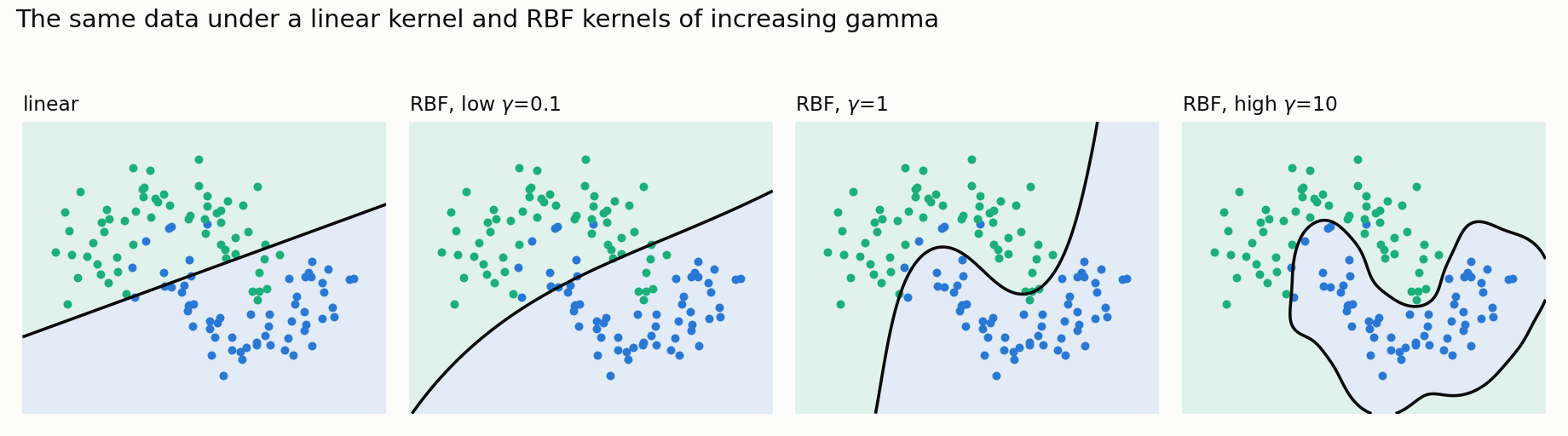
Because the two interact, tune them jointly on a logarithmic grid with cross-validation, on scaled features:

from sklearn.pipeline import make_pipeline
from sklearn.preprocessing import StandardScaler
from sklearn.svm import SVC
from sklearn.model_selection import GridSearchCV

pipe = make_pipeline(StandardScaler(), SVC(kernel="rbf"))
grid = GridSearchCV(
    pipe,
    {"svc__C": [0.1, 1, 10, 100], "svc__gamma": [0.01, 0.1, 1, 10]},
    cv=5, scoring="f1_macro",
)
grid.fit(X, y)

Imbalance, Confidence, and Probabilities

A few more options connect directly to the math:

• Imbalanced classes: pass class_weight="balanced" to re-weight the hinge penalties by class frequency, and evaluate with F1 or PR-AUC rather than accuracy.
• Confidence scores: decision_function returns the signed value $\mathbf{w}\cdot\phi(\mathbf{x})+b$, a distance-like margin score. That is the SVM’s native output.
• Probabilities: an SVM does not natively produce calibrated probabilities. Enabling probability=True fits an extra Platt-scaling model by cross-validation, which adds cost and can even disagree slightly with decision_function. Turn it on only when calibrated probabilities are genuinely needed.
• Scale: for a large linear problem, LinearSVC or SGDClassifier (hinge loss) scale far better than a kernel SVC.

Multiclass SVM

The SVM objective is intrinsically binary. Libraries extend it with a reduction: one-vs-one trains a classifier for every pair of classes and votes (scikit-learn’s SVC default), while one-vs-rest trains one classifier per class against all others. One-vs-one fits more, smaller problems; one-vs-rest fits fewer, larger ones. The choice affects training cost and calibration but not the underlying margin machinery.

Support Vector Regression

The same margin idea has a regression cousin, Support Vector Regression (SVR). It flips the hinge into an $\epsilon$-insensitive tube: errors smaller than $\epsilon$ cost nothing, and only points outside the tube (the support vectors) shape the fit. It inherits the kernel trick unchanged, so RBF-SVR fits smooth non-linear curves the same way RBF-SVC fits non-linear boundaries.

---

The dual and the kernel trick complete the two-class SVM. Part 4: One-Class SVM for Novelty Detection adapts the same margin-and-kernel machinery to deciding whether a point is normal at all.