Support Vector Machines, Part 4: One-Class SVM for Novelty Detection
One-Class SVM for novelty detection: the separating-from-the-origin objective, what the RBF unit-sphere property does and does not prove, and the roles of nu and gamma.
- Geometry, margins, and hinge loss
- The dual and support vectors
- The kernel trick
- One-Class SVM You are here
Part 1, Part 2, and Part 3 built the two-class SVM. This final part turns the same margin-and-kernel machinery to a different question: does a new point belong to a single “normal” class at all? That is novelty detection, and the One-Class SVM is its margin-based workhorse.
1. One-Class SVM for Novelty Detection
Of course. Outlier detection can be performed using One-Class SVM. It’s a powerful algorithm used for unsupervised outlier and novelty detection.
The core idea is simple and elegant: Instead of finding a hyperplane to separate two classes of data, a One-Class SVM learns a boundary that encloses a single class of data. Think of it as building a tight “fence” or “bubble” around the normal data points. Any point that falls outside this fence is then considered an outlier.
The Core Concept: From Separating Classes to Enclosing Data
Let’s quickly contrast it with a regular two-class SVM to understand the shift in thinking:
Regular SVM (Two Classes): Finds the widest possible street (margin) that separates Class A from Class B. The hyperplane is in the middle of the two classes.
One-Class SVM: Assumes all the training data belongs to one “normal” class. It then tries to find a hyperplane that separates these data points from the origin in a high-dimensional space, effectively creating a boundary around the data.
The goal is no longer to push two classes apart, but to define the territory of a single, “normal” class.
How It Works: The Mechanism
The algorithm is clever and relies heavily on the kernel trick.
Step 1: Map to a High-Dimensional Space (Kernel Trick)
First, the data is mapped from its original space into a very high-dimensional feature space using a kernel function. The RBF (Radial Basis Function) kernel is almost always used for this task. This mapping is crucial because it “unfolds” the data, making it possible to enclose even complex, non-spherical distributions with a simple hyperplane in the new space.
Step 2: Separate the Data from the Origin
In this feature space, the algorithm (the Schölkopf formulation) finds a hyperplane $\mathbf{w} \cdot \phi(\mathbf{x}) = \rho$ that pushes most of the mapped training points into the half-space $\mathbf{w} \cdot \phi(\mathbf{x}) \ge \rho$, as far from the origin as possible. Formally it solves:
\[\min_{\mathbf{w}, \rho, \xi} \; \frac{1}{2}\lVert \mathbf{w} \rVert^2 + \frac{1}{\nu n}\sum_{i} \xi_i - \rho \quad \text{subject to} \quad \mathbf{w} \cdot \phi(\mathbf{x}_i) \ge \rho - \xi_i, \; \xi_i \ge 0.\]The decision function is $f(\mathbf{x}) = \text{sign}(\mathbf{w} \cdot \phi(\mathbf{x}) - \rho)$: points scoring at or above $\rho$ are inliers, the rest outliers.
It is worth being precise about the geometry here, because the intuition is easy to get backwards. The learned object in feature space is a half-space, not a bubble. Most data lands on the $\ge \rho$ side; the feature-space origin scores $\mathbf{w} \cdot \mathbf{0} = 0 < \rho$, so the origin sits on the rejected side. The model separates the data from the origin; it does not wrap a boundary around the origin. The reason this looks like a closed “fence” around the normal data is that we view it back in the original input space: pulling the flat feature-space boundary back through a nonlinear kernel like the RBF bends it into a closed contour around the dense region. The closed shape is an artifact of the pullback, not of the feature-space geometry.
Step 3: Control the Boundary with the ν (Nu) Hyperparameter
We don’t need to define the margin width manually. Instead, we control the behavior of the algorithm with a single, powerful hyperparameter called ν (nu).
The ν parameter has a very intuitive meaning:
- It’s an upper bound on the fraction of training points that can be considered outliers (i.e., allowed to be outside the fence).
- It’s also a lower bound on the fraction of training points that will become support vectors (the points that actually define the fence).
These are genuine bounds from the optimization, not exact percentages guaranteed on any particular fit. Setting $\nu = 0.05$ says, roughly, “at most about 5% of training points should end up as margin errors (outliers), and at least about 5% will be support vectors,” with the exact counts subject to finite-sample size and the numerical solution. Treat $\nu$ as a dial for that trade-off, not a promise that exactly 95% of points fall inside.
Crucially, $\nu$ does not set the tightness of the boundary on its own. The kernel width $\gamma$ and the feature scaling matter just as much: a large $\gamma$ produces a wiggly boundary that hugs each point, a small one a smoother region, and because the RBF depends on distances, unscaled features distort the whole picture. In practice we tune $\nu$ and $\gamma$ together and scale the inputs first.
Using One-Class SVM for Outlier Detection
Here is the practical workflow for finding anomalies in new data.
Phase 1: Training
We train the One-Class SVM on a dataset that contains only (or mostly) normal, inlier data. For example:
- A dataset of thousands of successful, non-fraudulent credit card transactions.
- Sensor readings from a machine while it’s operating correctly.
During this phase, the SVM learns the shape of “normalcy” by building a boundary around these points.
Phase 2: Prediction
Now, we take a new, unseen data point and ask the model to classify it. The model calculates the point’s position relative to the learned boundary.
- If the model returns +1, it means the point falls inside the learned boundary. It is classified as an inlier (normal).
- If the model returns -1, it means the point falls outside the boundary, on the same side as the origin. It is flagged as an outlier or anomaly.
Example Application: We train a One-Class SVM on a month’s worth of normal factory machine vibrations. The model learns the boundary of these normal vibrations. The next day, a new vibration reading comes in.
- We feed this new reading to the trained model.
- The model returns -1.
- This signals an anomaly, alerting an operator that the machine’s behavior has deviated from the norm and may require maintenance.
Two Clarifications
First, what One-Class SVM estimates is a decision region capturing the support of the training distribution, not a minimum enclosing sphere. A closely related but distinct formulation, Support Vector Data Description (SVDD), does fit a minimum enclosing ball in feature space; for translation-invariant kernels like the RBF the two coincide under specific conditions, but they are not the same objective.
Second, One-Class SVM is fundamentally a novelty detection method: it assumes the training data are mostly clean and learns what “normal” looks like. It is often used for outlier detection too, which is fine, but if the training set is itself contaminated with anomalies, the learned boundary will stretch to include them, and detection degrades. Match the tool to whether the training data are clean.
2. When the Inliers Surround the Origin
In the original 2D space, if the inliers surround the origin, we cannot separate them from an origin they already contain. The solution is that the separation does not happen in the original space; it happens in the high-dimensional feature space created by the kernel.
The Paradox in the Original Space
Imagine our normal data forms a cloud centered on the origin, with an outlier further out (the left panel below). The One-Class SVM’s goal of “separating the data from the origin” looks impossible here: the origin sits right in the middle of the normal cloud, so no straight line can put the data on one side and the origin on the other.
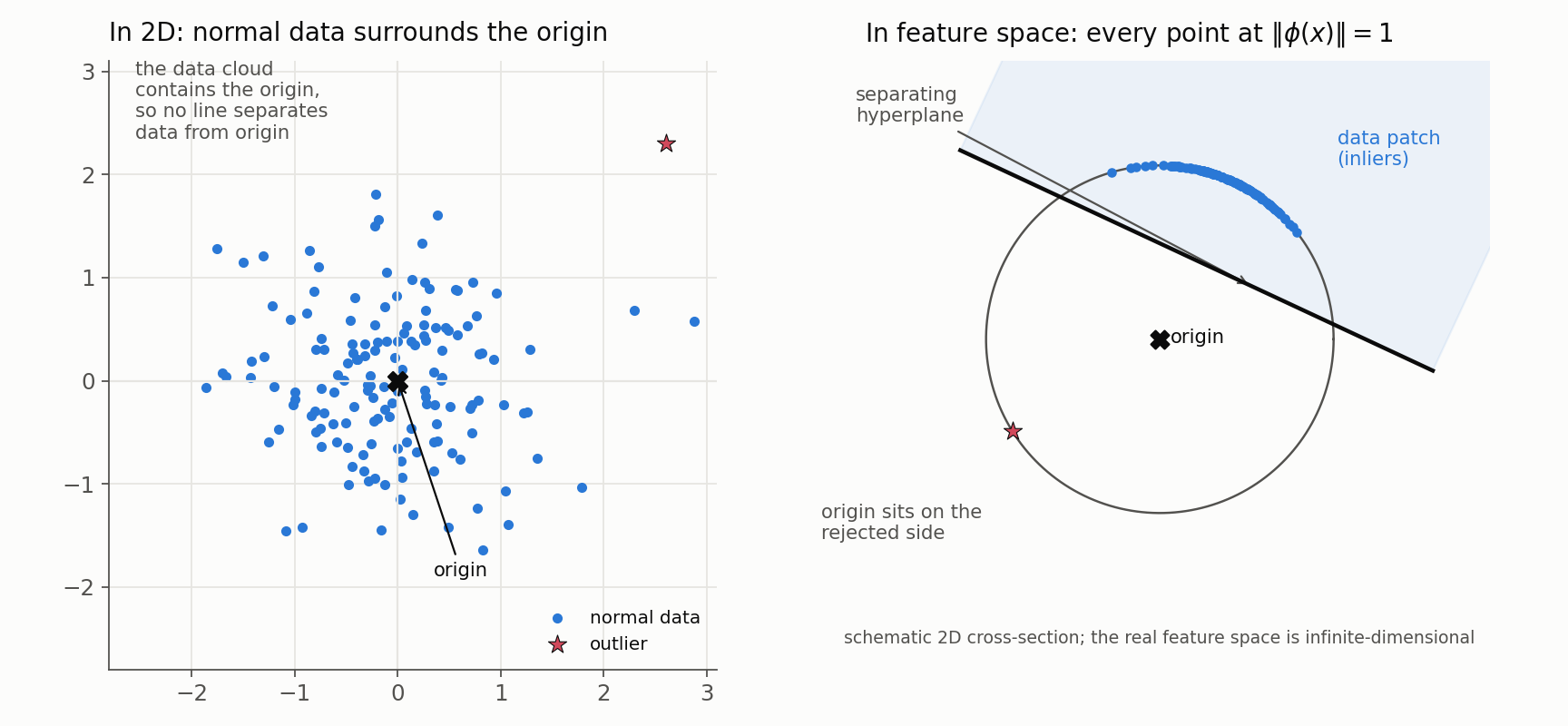
The right panel previews the fix, which the next subsection derives: the separation does not happen in the original space at all.
The Solution: The Magic of the Kernel Mapping
The kernel trick transforms the data so that this paradox is resolved. Let’s see how the commonly used RBF kernel $K(\mathbf{x}, \mathbf{z}) = \exp(-\gamma \lVert\mathbf{x} - \mathbf{z}\rVert^2)$ achieves this.
The kernel mapping, $\phi(\mathbf{x})$, takes our 2D points and projects them into an infinite-dimensional feature space. The crucial insight comes from looking at the distance of these new points from the origin in the new feature space.
The squared distance of a mapped point $\phi(\mathbf{x})$ from the feature space’s origin is $\lVert\phi(\mathbf{x})\rVert^2$. A key property of kernels is that this squared distance is equal to the kernel of the point with itself, $K(\mathbf{x}, \mathbf{x})$.
Let’s calculate this for the RBF kernel:
\[\|\phi(\mathbf{x})\|^2 = K(\mathbf{x}, \mathbf{x}) = \exp(-\gamma \|\mathbf{x} - \mathbf{x}\|^2)\] \[\|\phi(\mathbf{x})\|^2 = \exp(-\gamma \cdot 0) = \exp(0) = 1\]The “Aha!” Moment
This is a stunning result. It means that every single data point, regardless of its position in the original 2D space, is mapped to a new point that is exactly 1 unit away from the origin in the infinite-dimensional feature space.
The data that was a solid ball in 2D, including the origin, becomes the surface of a unit hypersphere in the feature space. The dense cluster of inliers is now a dense patch on the surface of this sphere.
Separating from the Origin in the Feature Space
Now, the problem is easy again!
- Data is Relocated: All our data points now live on a patch of a hollow shell (the unit hypersphere’s surface, since $\lVert\phi(\mathbf{x})\rVert = 1$ for the RBF kernel).
- Origin is Isolated: The origin of the feature space sits at the center of that shell, away from the patch of data on the surface.
- SVM Finds a Separating Half-Space: The One-Class SVM finds a hyperplane $\mathbf{w} \cdot \phi(\mathbf{x}) = \rho$ that puts the data patch on one side and leaves the origin (score 0) on the other. The learned region is the half-space containing the data, not a bubble drawn around the origin.
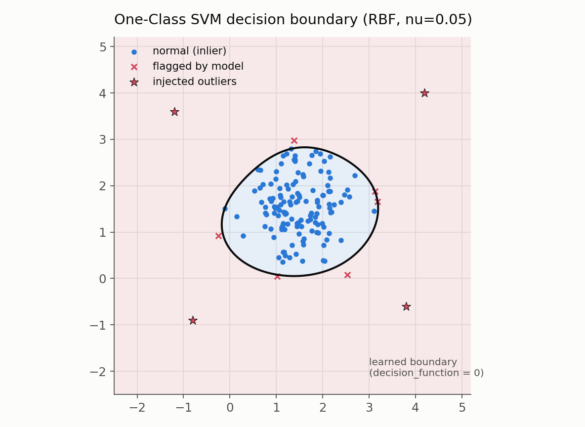
When that flat half-space boundary is mapped back down to the original 2D space, the nonlinear kernel bends it into the tight, closed contour (like a circle) around our inliers. The closed shape lives in input space; in feature space it is still just a half-space.
An Analogy: The Inflating Beach Ball
Imagine our 2D data is drawn on a completely deflated beach ball, with the inliers clustered around the center point (the future origin).
- The Kernel Trick is the process of inflating the ball.
- As we inflate it, our 2D drawing stretches and becomes the 3D surface of the ball.
- The Result: The center of the inflated ball (the 3D origin) is now empty. All of our data points are now on the surface, a set distance away from this new origin. The paradox is solved. The One-Class SVM can now easily find a boundary that separates the empty center from the data on the surface.
In summary, the kernel trick fundamentally rearranges the data’s geometry, ensuring that even if our inliers contain the origin in the original space, they are cleanly separated from the origin in the feature space, allowing the algorithm to work as intended.
3. The RBF Unit-Sphere Property and Its Limits
Yes, that is exactly right. This observation is at the core of understanding the RBF kernel’s power.
Irrespective of the positions of the data points in the original space, whether they are centered at the origin, far from it, or scattered everywhere, the RBF kernel maps every single point to the surface of a unit hypersphere in the high-dimensional feature space.
The Property Belongs to the Kernel, Not the Data
This seemingly magical property is a direct mathematical consequence of the RBF kernel’s definition, not the data’s layout. Let’s revisit the short derivation:
- The squared distance of a mapped point $\phi(\mathbf{x})$ from the origin in the feature space is $\|\phi(\mathbf{x})\|^2$.
- This is equal to the kernel of the point with itself: $K(\mathbf{x}, \mathbf{x})$.
- For the RBF kernel, $K(\mathbf{x}, \mathbf{x}) = \exp(-\gamma \lVert\mathbf{x} - \mathbf{x}\rVert^2)$.
- Since $\lVert\mathbf{x} - \mathbf{x}\rVert^2$ is always zero for any vector $\mathbf{x}$, the expression simplifies to $\exp(0) = 1$.
This proves that $\lVert\phi(\mathbf{x})\rVert^2 = 1$ for every point. The specific coordinates of $\mathbf{x}$ cancel themselves out, making the result universal for all points.
So, How Does It Differentiate Between Points?
This leads to the crucial follow-up question: If all points are just dumped onto the same sphere, how does the algorithm preserve the original data’s structure? How can it tell an inlier from an outlier?
Be careful about how much this proves, though. The unit-norm result says only that the points lie on the unit sphere of the feature space. It does not say they form a dense or complete spherical shell (they are a finite patch), that arbitrary arrangements become easy to separate, that original Euclidean distances are perfectly preserved, or that the points enclose the origin. What is preserved is a monotonic notion of pairwise closeness, while feature-space distances are nonlinearly bounded.
We can make this exact. The squared distance between two mapped points follows from the norms and the kernel:
\[\lVert \phi(\mathbf{x}_i) - \phi(\mathbf{x}_j) \rVert^2 = K(\mathbf{x}_i, \mathbf{x}_i) + K(\mathbf{x}_j, \mathbf{x}_j) - 2K(\mathbf{x}_i, \mathbf{x}_j) = 2 - 2K(\mathbf{x}_i, \mathbf{x}_j),\]using $K(\mathbf{x}, \mathbf{x}) = 1$ for the RBF. So pairwise feature-space distance is a direct, decreasing function of kernel similarity, and it saturates at $\sqrt{2}$ as points move far apart in the original space:
- Points close in original space: $\lVert\mathbf{x}_i - \mathbf{x}_j\rVert^2$ is small, so $K(\mathbf{x}_i, \mathbf{x}_j) \approx 1$ and the feature-space distance is near 0. They map close together on the sphere.
- Points far apart in original space: $K(\mathbf{x}_i, \mathbf{x}_j) \approx 0$, so the feature-space distance approaches $\sqrt{2}$, the maximum. They map to nearly orthogonal points. Notice this is bounded: no matter how far apart two points are in input space, their images never exceed distance $\sqrt{2}$.
The One-Class SVM then works on this hypersphere, finding the densest cluster of points and drawing a boundary (a hyperplane that intersects the sphere) around them. Outliers are simply points on the sphere that are far away from this dense cluster.
An Analogy: The World Map
Think of it like this:
- Original Space: Our 2D data is like a flat map of the world. Cities are at different
(x, y)coordinates. - Kernel Mapping: The RBF kernel acts like a projection that wraps this flat map onto a 3D globe.
- The Unit Hypersphere Property: Every city, whether it’s Bengaluru or New York, now lies on the surface of the globe. All cities are now approximately the same distance from the center of the Earth.
- Preserving Relative Positions: Relative closeness is preserved in a monotonic sense. Bengaluru and Chennai stay near each other on the globe’s surface; Bengaluru and New York stay far apart (though, as the $\sqrt{2}$ saturation above shows, “far” is capped once cities are beyond a certain distance).
- Finding the Boundary: The One-Class SVM’s job is to find a boundary (like a circle drawn on the globe’s surface) that encloses the dense cluster of “normal” cities, correctly identifying a remote, isolated city as an outlier.
A caveat on this picture: the globe (and the beach-ball earlier) is a finite 3D surface, whereas the RBF feature space is infinite-dimensional and only the equations above capture its geometry faithfully. Treat these analogies as intuition for “distances get bounded and rearranged,” not as a literal embedding.
4. One-Class SVM in Practice
Putting the pieces together: we train on data that is mostly normal, let the model learn the region, and flag anything scoring below the boundary. Viewed back in the input space, that boundary is the closed contour we expected, even though in feature space it is the flat separating half-space from Section 1.
1
2
3
4
5
6
7
8
9
10
11
12
13
14
import numpy as np
from sklearn.svm import OneClassSVM
from sklearn.pipeline import make_pipeline
from sklearn.preprocessing import StandardScaler

# fit preprocessing on the training partition only
oc = make_pipeline(
    StandardScaler(),
    OneClassSVM(kernel="rbf", gamma=0.3, nu=0.05),
).fit(X_train)

pred = oc.predict(X_test)                       # +1 inlier, -1 outlier
scores = oc.decision_function(X_test)           # signed; higher = more normal
sv_frac = oc[-1].support_.size / len(X_train)   # >= nu, per the nu-property
Fit the scaler on the training partition only, never on the test anomalies, or the tightness of the boundary leaks information. As Section 1 stressed, $\nu$ and $\gamma$ must be chosen together: $\nu$ bounds the outlier and support-vector fractions, while $\gamma$ sets how tightly the contour wraps the data.
Choosing a Threshold Without Many Anomaly Labels
Novelty detection rarely comes with a labeled anomaly set. In practice we either accept the $\nu$-implied boundary, or, when a small validation set of known anomalies exists, rank points by decision_function and pick the threshold that hits an acceptable precision/recall trade-off. Report the score distribution, not just the binary labels.
Where One-Class SVM Fits Among the Alternatives
It is one of several density- or geometry-based detectors, each with a different bias:
| Method | Core idea | Best when |
|---|---|---|
| One-Class SVM | Separate data from the origin in RBF space | Smooth, roughly unimodal normal region; clean training |
| Isolation Forest | Anomalies are easy to isolate by random splits | Higher dimensions, mixed feature types, some contamination |
| Local Outlier Factor | Compare a point’s local density to its neighbors | Varying-density clusters, local anomalies |
| SVDD | Minimum enclosing ball in feature space | When a bounding-volume view is more natural |
Failure Modes
One-Class SVM is not a universal detector. Watch for:
- High dimensionality: distances concentrate, and the RBF boundary becomes hard to tune.
- Multimodal normal data: a single smooth region fits several well-separated clusters poorly; consider a mixture or a per-cluster model.
- Contaminated training data: anomalies in the training set pull the boundary outward, exactly the novelty-versus-outlier distinction from Section 1.
- Distribution drift: a boundary learned last month may not describe this month’s “normal”, so retrain on a rolling window.