Bid Landscaping, Part 2: From Win Curve to Bidding, Pacing, and Its Limits

Bid Landscaping series - Part 1: Learning the Win Curve from the Auctions We Lost · Part 2 (this post): From Win Curve to Bidding, Pacing, and Its Limits

Part 1 built the object: for a given context, the win curve $W(b)=\Pr(\text{win}\mid \text{bid } b)=1-S(b)$, estimated with Kaplan-Meier from wins (which reveal the clearing price exactly) and losses (right-censored at our bid). This part spends that curve: how it turns into a bid, a pace, and an offline forecast - and, just as importantly, the handful of ways it quietly lies if we trust it past its evidence.

A one-line notation refresher (Part 1 has the full derivation): $b$ is our bid; $P$ the market’s winning threshold; $W_x(b)=F_x(b)=\Pr(P\le b\mid x)$ the win curve for context $x$; $\hat p_{i,x}$ the probability mass (the jump in the fitted win curve) at observed threshold $t_i$; and $v(x)$ the value to us of winning.

1. From Win Curve to Budget-Aware Bidding and Pacing

Here is where the landscape earns its keep in a bid optimizer - though not where it is usually assumed to. Start with the pieces of the decision:

• $x$ is an auction context, such as property × device × hour.
• $N(x)$ is how many such opportunities we expect to see.
• $v(x)$ is the value to us of winning one of them.
• $P$ is the unknown winning threshold drawn by the market.
• $\theta$ represents the knobs of our bidding policy, which turn context $x$ into a bid.

For one auction, profit is $v(x)-P$ if our bid reaches the threshold, and zero if it does not. The indicator below is simply the on/off switch that encodes those two outcomes. Summing over contexts and averaging over all thresholds the market might produce gives total expected profit:

\[\Pi(\theta) = \sum_x N(x) \cdot \mathbb{E}_{P}\Big[ \big(v(x) - P\big) \cdot \mathbb{1}\{\text{Bid}(x;\theta) \ge P\} \Big]\]

Read it from the inside out: for a possible threshold $P$, ask whether the policy wins; if it does, keep the surplus $v(x)-P$; then average that result over the threshold distribution and multiply by opportunity volume.

The landscape provides that threshold distribution. For context $x$, define

\[F_x(p) = \Pr(P \le p \mid x) = W_x(p)\]

The expectation can now be written as an integral over only the prices our bid would beat:

\[\Pi(\theta) = \sum_x N(x) \int_{[0,\,\text{Bid}(x;\theta)]} \big(v(x) - p\big) \, dF_x(p)\]

This integral is just a weighted sum in compact notation: consider every possible clearing price up to our bid, multiply the profit at that price by how likely the price is, and add the pieces. For the fitted KM curve, which is a step function rather than a smooth density, the computation is literally the finite sum from Part 1’s worked example:

\[\hat{\Pi}(\theta) = \sum_x N(x) \sum_{t_i \le \text{Bid}(x;\theta)} \big(v(x)-t_i\big)\hat{p}_{i,x}\]

Here $\hat{p}_{i,x}$ is the probability mass - the jump in the win curve - at observed threshold $t_i$ for context $x$. The landscape therefore turns an abstract expectation over competition into numbers the optimizer can evaluate.

First, an honest disclaimer: where the landscape changes nothing

In an idealized second-price auction with no constraints, the landscape does not change the per-auction bid. To see why, temporarily imagine a smooth population-level threshold distribution with density $f$. For one opportunity, bidding $b$ gives expected profit

\[\Pi(b) = \int_0^b (v-p)f(p)\,dp\]

Increasing the bid by a tiny amount exposes us only to the thin slice of auctions whose threshold is near that new bid. Each newly won auction in that slice is worth $v$ and costs about $b$, so the marginal profit is:

\[\frac{d\Pi(b)}{db} = \big(v - b\big) \, f(b)\]

The density $f(b)$ says how many extra auctions become winnable at that price; $v-b$ says whether each extra win is profitable. Below value, both pieces make increasing the bid worthwhile. Above value, every marginal win loses money. Thus the sign flips at $b=v$, giving $b^\star=v$: bid the value, whatever the competition looks like. That is the classic truthful-bidding result. The landscape moves the expected profit, spend, and volume at that bid - it does not move the unconstrained second-price bid itself.

So why estimate it at all? Because no production system lives in that idealized world. The landscape starts driving decisions the moment any of the following enters - and at least one always does.

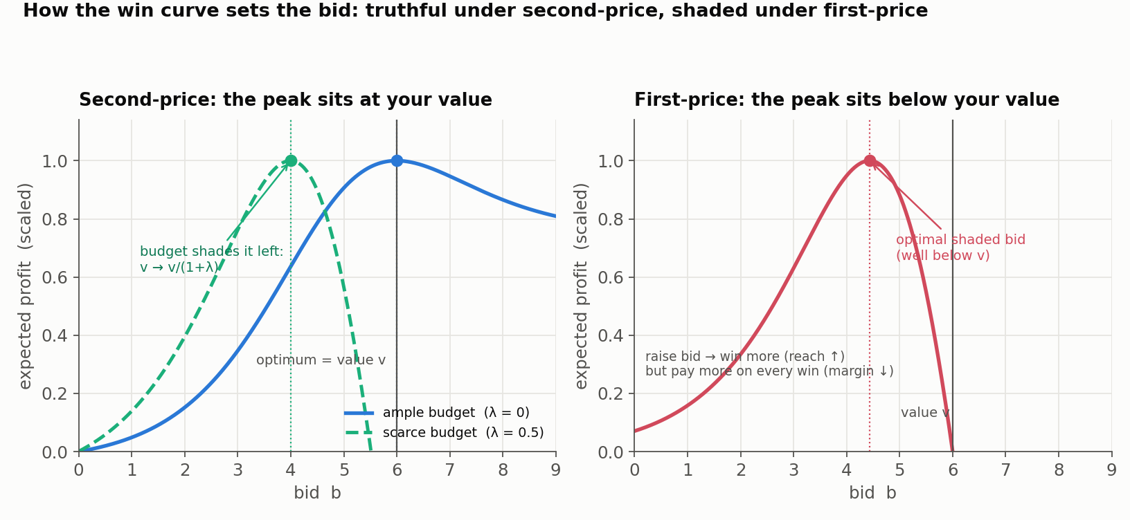
1. Budgets and pacing. With a budget, we can no longer afford to win everything worth winning. A Lagrange multiplier $\lambda \ge 0$ acts as the campaign’s internal price of scarce budget: spending one real dollar now carries an additional shadow cost of $\lambda$ dollars because it consumes capacity that could have been used later. The surplus from winning at threshold $p$ changes from $v-p$ to $v-(1+\lambda)p$:

\[\max_b \int_{[0,b]} \big(v - (1 + \lambda)\, p\big) \, dF(p) \quad \Rightarrow \quad b^\star = \frac{v}{1 + \lambda} \quad \text{(in the smooth idealization)}\]

When budget is plentiful, $\lambda=0$ and the formula returns the truthful bid $b^\star=v$. As budget becomes scarcer, $\lambda$ rises and the bid is shaded downward. The landscape does not create the scaling rule; it tells the pacing system which $\lambda$ will produce the required spend and volume across all contexts. This is the use I first met at Walmart, working on campaign budget underutilization: “how much more volume does a 10% bid increase buy?” is a question about the slope of the win curve, and pacing tolerates a coarse landscape, which makes it the ideal first consumer of one.

2. Counterfactual / off-policy evaluation. Before deploying a new bidding policy, the landscape predicts its win rate, spend, and profit offline. One discipline applies: this works for bids inside the support of our data. Asking for $W(4.50)$ when our observations span \$2-\$7 is interpolation; asking what happens at \$55 when our bids never exceeded \$50 is tail extrapolation, and non-parametric KM is flat and silent past its last observation (caveat 1 below). The landscape evaluates counterfactuals we have evidence about, not arbitrary ones.

3. First-price auctions and bid shading. Where we pay our own bid, a win at bid $b$ produces profit $v-b$, regardless of how far below $b$ the hidden threshold was. Because $F(b)$ is the probability that the threshold falls below our bid, expected profit becomes

\[\Pi_{\text{first-price}}(b) = F(b)(v-b)\]

Now raising the bid has two opposing effects: it increases $F(b)$ and therefore wins more auctions, but it also reduces $v-b$ on every auction won at that bid. The best bid balances reach against margin, so the shape of the landscape directly controls shading. Estimating that landscape still requires the right feedback: our first-price payment alone does not reveal the hidden threshold. We need threshold feedback from the platform or a current-status/interval-censored estimator built from win/loss observations at varied bids. ROI and CPA constraints, bid floors and caps, and the option to sit out create related trade-offs.

Putting the three regimes on one picture makes the role of the curve concrete. In a second-price auction the optimum sits at the value and only budget scarcity shades it left; in a first-price auction the optimum sits below the value, because a higher bid erodes margin on every win, and the whole balance is set by the shape of the landscape:

And the point worth stating precisely: the estimated $F(p)$ inside all of these must be censoring-aware. Under the feedback assumed in Part 1, lost auctions participate by shrinking the KM risk set. Under win/loss-only feedback, they instead enter a current-status likelihood. Either route removes the specific survivorship error of discarding losses, but that is not the same as being fully unbiased: censoring-awareness alone does not cure confounded bids, policy drift, or context mixing; those need the assumptions in the next section. (This censoring-aware view of bid landscapes is well established in the RTB literature - it underpins bid-aware gradient descent from KDD 2016 and the Deep Landscape Forecasting model from KDD 2019, which wires survival reasoning into an RNN.)

2. Reading the Curve Honestly: Caveats

A KM bid landscape is only as trustworthy as the data feeding it. Five things to respect:

1. The tail is unresolved. Our highest record in Part 1’s toy (auction 6 at \$7) was a loss - censored. That loss proves some threshold mass lies above \$7, but tells us nothing about where in the tail it lies. The KM estimate therefore remains flat at 0.625 beyond its last observed event; it cannot resolve the curve’s shape above \$7. To learn the top of the curve, we must occasionally bid higher.

2. We need bid spread to trace the whole curve. If every auction had been bid at exactly \$5, the exact prices on wins would still let us estimate the curve below \$5, and the losses would tell us how much probability mass remains above it. But we would learn nothing about how that upper-tail mass is distributed. Variation in bids (across time, across contexts, or via deliberate exploration) moves the censoring boundary and reveals higher parts of the landscape.

3. Endogeneity is the make-or-break. KM assumes the censoring point (our bid) is independent of the clearing price - non-informative censoring. In reality we bid high exactly where and when we judge value high, which often correlates with stiffer competition. Fit naively on such observational data and we get a biased, too-flat curve (“bid more, didn’t win proportionally more” - because competition was also higher then).

   The highest-leverage mitigation is a small exploration budget: randomly perturb the deployed bid by ±ε on a slice of traffic. That gives clean, unconfounded variation and turns the landscape from suggestive into trustworthy. But “perturb by ±ε” is a research sketch, not a production design - a real exploration policy needs eligible/safe traffic only, a logged randomization probability (so the exploration is analyzable after the fact), bid and budget caps, enough variation across the support to actually identify the curve, monitoring for advertiser and publisher harm, awareness that our own perturbation can move the market (interference), and a rollback rule. And note the scope of what it buys: small perturbations identify the local response near the deployed bid; they do not reveal the far tail (caveat 1). The assumption we actually need is not unconditional independence ($P \perp B$) but conditional independence ($P \perp B \mid X$): after conditioning on auction context $X$, our bid should carry no additional information about the threshold. That is the real argument for estimating landscapes per segment, and it trades directly against caveat 5: condition on too much context and every segment becomes too sparse to estimate.

4. Match the estimator to what we actually log. Part 1’s worked example assumed we observe the exact winning threshold on wins - textbook right-censored KM. In the clean second-price case that threshold equals the price paid, but this is not generally true in a first-price or rank-adjusted auction. If we have only a win/loss flag at our bid, the data is “current-status” and the correct tool is isotonic regression / NPMLE (pool-adjacent-violators on the win indicator versus bid) - the same monotone-curve idea, but different machinery that leans much harder on bid spread. Use KM only when the logged win feedback genuinely reveals the threshold.

5. Sparsity and non-stationarity. Estimate at a coarse enough grain to have volume (ad-group, or property × device - not the full joint context), over a window short enough that competition hasn’t shifted, and re-estimate on a slow loop. Competitors adapt; a landscape is a perishable artifact, never a frozen one.

One more practical note from the hotel-ads world: some platforms won’t give us auction-level win/loss logs at all, but expose a bid simulator instead - a per-criterion curve of estimated clicks, cost, and impressions at alternative bids. In our language, that is an operational analogue of the landscape, pre-built by the platform from the full auction data we never see - including the lost auctions and the competitors’ bids. One caution on reading it: $\text{clicks}(b)$ is not literally the win curve. Clicks fold together eligibility, auction wins, position effects, and click-through - roughly $N \cdot P(\text{win} \mid b) \cdot \mathbb{E}[\text{CTR} \mid \text{won}, b]$ - so simulator curves are downstream response curves, one step removed from the pure auction-level $W(b)$. They still serve the pacing and counterfactual jobs well. Using them largely sidesteps the endogeneity problem in caveat 3, at the price of inheriting a model we cannot audit - so backtest the simulator’s predicted point against our realized clicks and cost before trusting it for budget decisions.

Choosing the estimator by what we log

The right tool follows mechanically from the feedback the platform gives us:

Logged feedback	Right tool
Exact winning threshold on wins + our bid on losses	Kaplan-Meier (Part 1)
Only a win/loss flag at our bid	Current-status NPMLE / isotonic regression
Exact market price for every auction	Plain empirical CDF - no censoring machinery needed
High volume + rich context	Conditional survival models (below)
Strong temporal drift	Rolling / time-weighted re-estimation

We have name-dropped the win/loss-only tools twice now, so a short orientation on each is owed.

Isotonic regression is curve fitting with a single constraint: the fitted curve may never decrease. Feed it (bid, won?) pairs and it finds the non-decreasing step function that best fits the outcomes in a least-squares sense. The classic algorithm, pool-adjacent-violators (PAVA), is almost mechanical: sort auctions by bid, compute the raw win rate at each bid level, and wherever a rate drops as the bid rises - a violation, since a true win curve cannot decrease - merge the offending neighbors and replace both with their pooled average. Repeat until no violations remain. What survives is a monotone staircase $\hat{W}(b)$ built from nothing but flags: no threshold prices required, which is exactly why it fits the feedback-poor regime.

NPMLE (non-parametric maximum likelihood estimation) reaches the same destination from the likelihood side. Treat the entire threshold distribution $F$ as the unknown, assuming no parametric shape: a win at bid $b$ says the threshold sat below our bid and contributes likelihood $F(b)$; a loss says the opposite and contributes $1 - F(b)$. Maximize the product over all possible distributions and, for this win/loss-at-a-bid (“current status”) data, the maximizer turns out to be computed exactly by PAVA - the optimization view and the likelihood view are two doors into the same estimator. The connection runs deeper still: Kaplan-Meier is itself the NPMLE for right-censored data, so the first two rows of the table differ not in philosophy but in how much each observation reveals.

Both tools deserve the same end-to-end treatment KM received in Part 1 - a worked toy, the failure modes, the production caveats. The seller-side twin of this problem - a publisher setting floor prices, which turns on exactly these monotone win/loss-at-a-bid curves - is taken up in the floor-price bid-threshold classifiers article; the win/loss-only estimators here get their own dedicated treatment in future articles.

And when a single per-segment curve stops being enough, there is a natural ladder to climb, each rung buying more context-sensitivity at the price of more data and more assumptions: global KM, then stratified KM (one curve per segment), then semi-parametric conditional models (Cox, accelerated failure time), then tree ensembles (random survival forests, gradient-boosted survival), and finally neural conditional models like Deep Landscape Forecasting. Climb only as far as volume supports. The toy in Part 1 is rung one - and rung one estimated correctly beats rung five fed with wishful data.

3. The Money and Power Ledgers

Like the rest of this series, the landscape is worth reading through two ledgers - one tracking money, one tracking data and who holds the informational upper hand.

Money ledger. It is easy to conflate the four different numbers a single won auction touches, so name them explicitly (using Part 1’s toy; all per-impression here; multiply by 1000 for the CPM the exchange usually quotes, and note whether each figure is gross or net of fees):

Quantity	In the toy	What it is
Effective winning threshold $P$	\$5 (at the \$5 rung)	What the market demanded - recovered by KM
Our submitted bid $b$	\$6 on those wins	The lever we set
Payment on a win	the clearing price $\le b$	Second-price: we pay $P$, not $b$
Expected cost per win	\$4.00 at $b=5$	Mass-weighted over won prices, not the raw win average
Budget debit	payment (+ any DSP fee)	What the pacing loop actually decrements

The gap between bid, threshold, and payment is the whole reason the landscape exists: a value-only bidder sees none of these three as distinct.

Data / privacy and power ledger. The landscape is unusually privacy-light for something this valuable. It is conditioned on auction context $x$ - query, device, geography, hour, placement - none of which requires a persistent cross-user identifier; a bid landscape can be estimated almost entirely contextually. What it does need is an auction-outcome log retained over a window long enough to fit but short enough to stay fresh (caveat 5), with the usual access controls on competitive pricing data. Exploration (caveat 3) is the one step that changes exposure: deliberately perturbing bids alters what advertisers pay and what publishers earn on that slice of traffic, so its blast radius belongs in the ledger, not just the methodology.

The sharpest entry, though, is power. The platform running the auction sees every bid from every participant, won or lost; the advertiser sees only its own wins and losses, and often not even those - just an aggregated bid simulator curve (the bid-simulator caveat above) built from data it will never hold. That asymmetry is structural: the whole reason we reach for survival analysis is that we are reconstructing, from censored fragments, a distribution the auctioneer observes directly. KM narrows the gap; it does not close it.

4. Recap

The win curve Part 1 built honestly is what this part spent. Four uses, one warning:

• Second-price bidding: the landscape moves expected profit, spend, and volume - but leaves the unconstrained bid at the value, $b^\star=v$.
• Budgets and pacing: a shadow price $\lambda$ shades the bid to $v/(1+\lambda)$, and the landscape tells the pacing loop which $\lambda$ hits the target spend.
• First-price shading: here the curve does set the bid, trading reach $F(b)$ against margin $v-b$, with the optimum below value.
• Offline evaluation: the landscape forecasts a new policy’s win rate, spend, and profit - but only for bids inside the support of our data.

The warning is the five caveats: a KM landscape is censored, endogenous, and perishable, and reading it past its evidence - into the unresolved tail, or as if our bids were unconfounded - quietly lies. The medical statisticians who built this machinery in 1958 were trying not to lie about patients who left the study early. The same discipline - refusing to invent data we didn’t observe, while refusing to throw away the partial information we did - is exactly what separates a bid optimizer that learns from the full market from one that studies only the planes that came back.

References

• Kaplan, E. L. & Meier, P. (1958). Nonparametric Estimation from Incomplete Observations. JASA.
• Zhang, W. et al. (2016). Bid-aware Gradient Descent for Unbiased Learning with Censored Data in Display Advertising. KDD 2016. (ACM DL)
• Ren, K. et al. (2019). Deep Landscape Forecasting for Real-time Bidding Advertising. KDD 2019. (arXiv:1905.03028)
• Ghosh, A. et al. (2019). Scalable Bid Landscape Forecasting in Real-time Bidding. ECML-PKDD 2019. (arXiv:2001.06587)